The use of the derivative in various fields of activity. An interesting derivative The objectives of this work: To consider the use of the derivative in various sciences To get acquainted with scientists who have studied the derivative of a function. Force is the derivative of work in displacement.

Ministry of Education Saratov region

State Autonomous Professional educational institution Saratov region "Engels Polytechnic"

APPLICATION OF THE DERIVATIVE IN DIFFERENT FIELDS OF SCIENCE

Performed: Sarkulova Nurgulya Sergeevna

student of group KShI-216/15

(Design, modeling and

sewing technology)

scientific adviser:

Verbitskaya Elena Vyacheslavovna

teacher of mathematics GAPOU SO

"Engels Polytechnic"

2016

Introduction

The role of mathematics in various fields of natural science is very great. No wonder they say“Mathematics is the queen of sciences, its physics right hand, chemistry is left.

The subject of research is the derivative.

The leading goal is to show the significance of the derivative not only in mathematics, but also in other sciences, its importance in modern life.

Differential calculus is a description of the world around us, made in mathematical language. The derivative helps us successfully solve not only math problems, but also practical tasks in various fields of science and technology.

The derivative of a function is used wherever there is an uneven process flow: this is an uneven mechanical movement, and alternating current, and chemical reactions and radioactive decay substances, etc.

Key and thematic questions of this essay:

1. The history of the origin of the derivative.

2. Why study derivatives of functions?

3. Where are derivatives used?

4. Application of derivatives in physics, chemistry, biology and other sciences.

5. Conclusions

I decided to write a paper on the topic "Application of the derivative in various fields of science", because I think this topic is very interesting, useful and relevant.

In my work, I will talk about the application of differentiation in various fields of science, such as chemistry, physics, biology, geography, etc. After all, all sciences are inextricably linked, which is very clearly seen in the example of the topic I am considering.

Application of the derivative in various fields of science

From the high school algebra course, we already know that derivative is the limit of the ratio of the increment of the function to the increment of its argument as the increment of the argument tends to zero, if such a limit exists.

The action of finding a derivative is called its differentiation, and a function that has a derivative at a point x is called differentiable at that point. A function that is differentiable at each point on an interval is called differentiable on that interval.

The honor of discovering the basic laws of mathematical analysis belongs to English physicist and the mathematician Isaac Newton and the German mathematician, physicist, philosopher Leibniz.

Newton introduced the concept of a derivative, studying the laws of mechanics, thereby revealing its mechanical meaning.

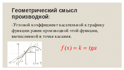
The physical meaning of the derivative: the derivative of a functiony= f(x) at the point x 0 is the rate of change of the functionf(x) at the point x 0 .

Leibniz came to the concept of a derivative by solving the problem of drawing a tangent to a derivative line, thus explaining it geometric meaning.

The geometric meaning of the derivative is that the derivative function at a pointx 0 equal to the slope of the tangent to the graph of the function drawn at the point with the abscissax 0 .

The term derivative and modern notationy" , f"Introduced by J. Lagrange in 1797.

Russian mathematician In the 19th century, Panfuty Lvovich Chebyshev said that "of particular importance are those methods of science that allow us to solve a problem common to all practical human activity, for example, how to dispose of our means to achieve the greatest benefit."

Representatives of various specialties have to deal with such tasks in our time:

Process engineers try to organize production in such a way that as many products as possible are produced;

Designers are trying to develop a device for spaceship so that the mass of the device is the smallest;

Economists try to plan the links between the plant and the sources of raw materials in such a way that transportation costs are minimal.

When studying any topic, students have a question: “Why do we need this?” If the answer satisfies curiosity, then we can talk about the interest of the students. The answer for the topic "Derivative" can be obtained by knowing where derivatives of functions are used.

To answer this question, we can list some disciplines and their sections in which derivatives are used.

Derivative in algebra:

1. Tangent to the function graph

Tangent to function graphf, differentiable at x about , is a line passing through the point (x about ; f(x o )) and having a slopef′(x o ).

y= f(x o ) + f′(x o ) (x - x o )

2. Search for intervals of increasing and decreasing functions

Functiony=f(x) increases over the intervalX , if for any andthe inequality. In other words, a larger value of the argument corresponds to a larger value of the function.

Functiony=f(x) decreases over the intervalX , if for any andthe inequality. In other words, a larger value of the argument corresponds to a smaller value of the function.

3. Finding extremum points of a function

point calledmaximum point functionsy=f(x) if for allx . The value of the function at the maximum point is calledfunction maximum and denote.

point calledminimum point functionsy=f(x) if for allx from its neighborhood the inequality. The value of the function at the minimum point is calledfunction minimum and denote.

Under the neighborhood of a point understand interval, where is a small enough positive number.

The minimum and maximum points are calledextremum points , and the function values corresponding to the extremum points are calledfunction extrema .

4. Search for intervals of convexity and concavity of a function

Function Graph, is on this intervalconvex , lies no higher than any of its tangents (Fig. 1).

Function Graph, differentiable on the interval, is on this intervalconcave , if the graph of this function is within the interval lies not lower than any of its tangents (Fig. 2).

The inflection point of the function graph is called the point separating the intervals of convexity and concavity.

5. Finding the inflection points of a function

Derivative in physics:

1. Speed as a derivative of the path

2. Acceleration as a derivative of speeda =

3. Decay rate radioactive elements 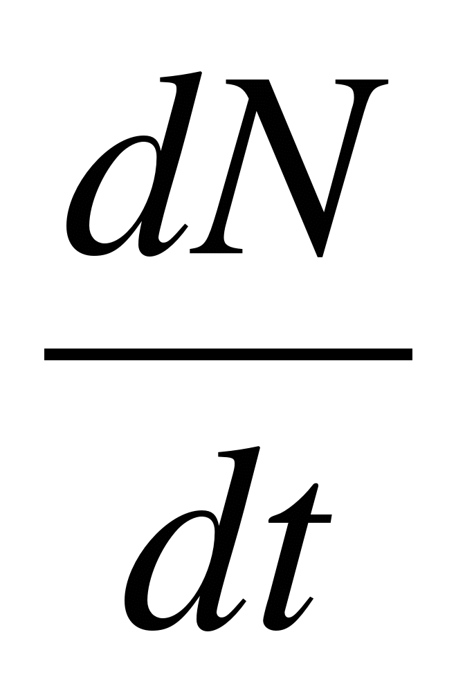= - λN

And also in physics, the derivative is used to calculate:

Speeds material point

Instantaneous speed as the physical meaning of the derivative

Instant value AC power

Instantaneous value of the EMF of electromagnetic induction

Max Power

Derivative in chemistry:

And in chemistry, differential calculus has found wide application for constructing mathematical models chemical reactions and the subsequent description of their properties.

The derivative in chemistry is used to determine a very important thing - speed chemical reaction, one of the decisive factors that must be taken into account in many areas of scientific and industrial activity. V(t) = p'(t)

Quantity

in-va at a time t 0

p = p(t 0 )

Function

Time interval

∆t = t– t 0

Argument Increment

Change in quantity

∆p=p(t 0 + ∆t) – p(t 0 )

Function increment

Average rate of a chemical reaction

∆p/∆t

Ratio of function increment to argument increment

Derivative in biology:

A population is a set of individuals of a given species occupying a certain area of the territory within the range of the species, freely interbreeding with each other and partially or completely isolated from other populations, and is also an elementary unit of evolution.

P \u003d x‘ (t)

Derivative in geography:

1. Some meanings in seismography

2. Features electromagnetic field land

3. Radioactivity of nuclear geophysical indicators

4. Many meanings in economic geography

5. Derive a formula for calculating the population in the territory at time t.

y'= to y

The idea of the sociological model of Thomas Malthus is that population growth is proportional to the population at a given time t through N(t). The Malthus model worked well for describing the US population from 1790 to 1860. This model is no longer valid in most countries.

Derivative in electrical engineering:

In our homes, in transport, in factories: electric current works everywhere. Under the electric current understand the directed movement of free electrically charged particles.

Quantitative characteristic electric current is the current strength.

In an electric circuit electric charge changes over time according to the law q=q (t). The current I is the derivative of the charge q with respect to time.

In electrical engineering, AC operation is mainly used.

Electric current that changes with time is called alternating current. The AC circuit may contain various elements: heating devices, coils, capacitors.

The production of alternating electric current is based on the law of electromagnetic induction, the formulation of which contains the derivative of the magnetic flux.

Derivative in economics:

Economics is the basis of life, and differential calculus, an apparatus for economic analysis, occupies an important place in it. The basic task of economic analysis is to study the relationships of economic quantities in the form of functions.

The derivative in economics solves important questions:

1. In what direction will the state's income change with an increase in taxes or with the introduction of customs duties?

2. Will the company's revenue increase or decrease with an increase in the price of its products?

To solve these questions, it is necessary to construct the connection functions of the input variables, which are then studied by the methods of differential calculus.

Also, using the extremum of the function (derivative) in the economy, you can find the highest labor productivity, maximum profit, maximum output and minimum costs.

CONCLUSION: the derivative is successfully used in solving various applied problems in science, technology and life

As can be seen from the above, the use of the derivative of a function is very diverse, and not only in the study of mathematics, but also in other disciplines. Therefore, we can conclude that the study of the topic: "The derivative of a function" will have its application in other topics and subjects.

We were convinced of the importance of studying the topic "Derivative", its role in the study of the processes of science and technology, the possibility of designing according to real events mathematical models, and solve important problems.

“Music can uplift or soothe the soul,
Painting is pleasing to the eye,
Poetry - to awaken feelings,
Philosophy - to satisfy the needs of the mind,
Engineering is to improve the material side of people's lives,
BUTmathematics can achieve all these goals.”

So said the American mathematicianMaurice Kline.

Bibliography:

1. Bogomolov N.V., Samoylenko I.I. Maths. - M.: Yurayt, 2015.

2. V. P. Grigoriev and Yu. A. Dubinsky, Elements of Higher Mathematics. - M.: Academy, 2014.

3. Bavrin I.I. Fundamentals of higher mathematics. - M.: graduate School, 2013.

4. Bogomolov N.V. Practical lessons in mathematics. - M.: Higher school, 2013.

5. Bogomolov N.V. Collection of problems in mathematics. - M.: Bustard, 2013.

6. Rybnikov K.A. History of mathematics, Moscow University Press, M, 1960.

7. Vinogradov Yu.N., Gomola A.I., Potapov V.I., Sokolova E.V. – M.:Publishing Center "Academy", 2010

8 . Bashmakov M.I. Mathematics: algebra and the beginnings of mathematical analysis, geometry. - M.: Publishing Center "Academy", 2016

Periodic sources:

Newspapers and magazines: "Mathematics", " Public lesson»

Use of Internet resources, digital libraries:

www:egetutor.ru

matematika-na5.norod.ru

FGOU SPO

Novosibirsk agricultural college

abstract

in the discipline "mathematics"

"Application of the derivative in science and technology"

S. Razdolnoe 2008

Introduction

1. Theoretical part

1.1 Problems leading to the concept of a derivative

1.2 Derivative definition

1.3 General rule for finding the derivative

1.4 Geometric meaning of the derivative

1.5 Mechanical meaning of the derivative

1.6 Second order derivative and its mechanical meaning

1.7 Definition and geometric meaning of the differential

2. Investigation of functions with the help of the derivative

Conclusion

Literature

Introduction

In the first chapter of my essay, we will talk about the concept of a derivative, the rules for its application, about geometric and physical sense derivative. In the second chapter of my essay, we will talk about the use of the derivative in science and technology and about solving problems in this area.

1. Theoretical part

1.1 Problems leading to the concept of a derivative

When studying certain processes and phenomena, the problem often arises of determining the speed of these processes. Its solution leads to the concept of a derivative, which is the basic concept of differential calculus.

The method of differential calculus was created in the 17th and 18th centuries. The names of two great mathematicians, I. Newton and G.V. Leibniz.

Newton came to the discovery of differential calculus when solving problems about the speed of a material point at a given moment of time (instantaneous speed).

As is known, uniform movement is a movement in which a body travels equal lengths of the path in equal intervals of time. The distance traveled by a body in a unit of time is called speed uniform motion.

However, most often in practice we are dealing with uneven movement. A car driving on the road slows down at the crossings and speeds it up in those sections where the path is clear; the aircraft slows down when landing, etc. Therefore, most often we have to deal with the fact that in equal time intervals the body passes path segments of different lengths. Such a movement is called uneven. Its speed cannot be characterized by a single number.

Often, to characterize uneven motion, the concept is used average speed movement during the time ∆t٫ which is determined by the relation where ∆s is the path traveled by the body during the time ∆t.

So, with a body in free fall, the average speed of its movement in the first two seconds is

In practice, such a characteristic of movement as average speed says very little about movement. Indeed, at 4.9 m / s, and for the 2nd - 14.7 m / s, while the average speed for the first two seconds is 9.8 m / s. The average speed during the first two seconds does not give any idea of how the movement occurred: when the body moved faster, and when slower. If we set the average speeds of movement for each second separately, then we will know, for example, that in the 2nd second the body moved much faster than in the 1st. However, in most cases much faster than we are not satisfied with. After all, it is easy to understand that during this 2nd second the body also moves in different ways: at the beginning it is slower, at the end it is faster. And how does it move somewhere in the middle of this 2nd second? In other words, how to determine the instantaneous speed?

Let the motion of the body be described by the law for a time equal to ∆t. At the moment t0 the body has passed the path, at the moment - the path. Therefore, during the time ∆t, the body has traveled a distance and the average speed of the body over this period of time will be.

The shorter the time interval ∆t, the more accurately it is possible to establish with what speed the body is moving at the moment t0, since a moving body cannot significantly change its speed in a short period of time. Therefore, the average speed as ∆t tends to zero approaches the actual speed of movement and, in the limit, gives the speed of movement at a given time t0 (instantaneous speed).

In this way ,

Definition 1. Instant Speed of rectilinear motion of the body at a given time t0 is called the limit of the average speed over the time from t0 to t0+ ∆t, when the time interval ∆t tends to zero.

So, in order to find the speed of rectilinear non-uniform motion at a given moment, it is necessary to find the limit of the ratio of the increment of the path ∆to the increment of time ∆t under the condition i.e. Leibniz came to the discovery of differential calculus while solving the problem of constructing a tangent to any curve given by his equation.

The solution to this problem has great importance. After all, the speed of a moving point is directed along a tangent to its trajectory, therefore, determining the speed of a projectile on its trajectory, the speed of any planet in its orbit, is reduced to determining the direction of the tangent to the curve.

The definition of a tangent as a straight line that has only one common point with a curve, which is valid for a circle, is unsuitable for many other curves.

The following definition of a tangent to a curve not only corresponds to the intuitive idea about it, but also allows you to actually find its direction, i.e. calculate the slope of the tangent.

Definition 2. Tangent to the curve at the point M is called the straight line MT, which is the limiting position of the secant MM1, when the point M1, moving along the curve, indefinitely approaches the point M.

1.2 Derivative definition

Note that when determining the tangent to the curve and the instantaneous speed of non-uniform motion, essentially the same mathematical operations are performed:

1. The given value of the argument is incremented and a new value of the function is calculated corresponding to the new value of the argument.

2. Determine the function increment corresponding to the selected argument increment.

3. The increment of the function is divided by the increment of the argument.

4. Calculate the limit of this ratio, provided that the increment of the argument tends to zero.

Solutions of many problems lead to limit transitions of this type. It becomes necessary to make a generalization and give a name to this passage to the limit.

The rate of change of the function depending on the change of the argument can obviously be characterized by a ratio. This relationship is called average speed function changes on the interval from to. Now we need to consider the limit of a fraction. The limit of this ratio as the increment of the argument tends to zero (if this limit exists) is some new function of. This function is denoted by the symbols y', called derivative this function, since it is obtained (produced) from the function The function itself is called primitive function with respect to its derivative

Definition 3. derivative functions at a given point name the limit of the ratio of the increment of the function ∆y to the corresponding increment of the argument ∆x, provided that ∆x→0, i.e.

1.3 General rule for finding the derivative

The operation of finding the derivative of some function is called differentiation functions, and the branch of mathematics that studies the properties of this operation is differential calculus.

If a function has a derivative at x=a, then it is said to be differentiable at this point. If a function has a derivative at every point in a given interval, then it is said to be differentiable On this interval .

The definition of the derivative not only fully characterizes the concept of the rate of change of a function when the argument changes, but also provides a way to actually calculate the derivative of a given function. To do this, you must perform the following four actions (four steps) indicated in the definition of the derivative itself:

1. Find a new function value by presenting in this function instead of x, the new value of the argument: .

2. The increment of the function is determined by subtracting the given value of the function from its new value: .

3. Compose the ratio of the increment of the function to the increment of the argument: .

4. Go to the limit at and find the derivative: .

Generally speaking, a derivative is a “new” function derived from a given function according to a specified rule.

1.4 Geometric meaning of the derivative

The geometric interpretation of the derivative, first given in late XVII in. Leibniz is as follows: the value of the derivative of the function at the point x is equal to the slope of the tangent drawn to the graph of the function at the same point x, those.

The equation of a tangent, like any straight line passing through given point in this direction, has the form – current coordinates. But the tangent equation will also be written as follows: . The normal equation will be written in the form

1.5 Mechanical meaning of the derivative

The mechanical interpretation of the derivative was first given by I. Newton. It consists in the following: the speed of movement of a material point at a given moment of time is equal to the derivative of the path with respect to time, i.e. Thus, if the law of motion of a material point is given by an equation, then to find the instantaneous velocity of a point at some particular moment in time, you need to find the derivative and substitute the corresponding value of t into it.

1.6 Second order derivative and its mechanical meaning

We get (an equation from what was done in the textbook Lisichkin V.T. Soloveychik I.L. "Mathematics" p. 240):

In this way, the acceleration of the rectilinear motion of the body at a given moment is equal to the second derivative of the path with respect to time, calculated for a given moment. This is the mechanical meaning of the second derivative.

1.7 Definition and geometric meaning of the differential

Definition 4. The main part of the increment of a function, linear with respect to the increment of the function, linear with respect to the increment of the independent variable, is called differential functions and is denoted by d, i.e. .

Function differential geometrically represented by the increment of the ordinate of the tangent drawn at the point M ( x ; y ) for given values of x and ∆x.

calculation differential – .

Application of the differential in approximate calculations – , the approximate value of the increment of the function coincides with its differential.

Theorem 1. If the differentiable function increases (decreases) in a given interval, then the derivative of this function is not negative (not positive) in this interval.

Theorem 2. If the derivative function is positive (negative) in some interval, then the function in this interval is monotonically increasing (monotonically decreasing).

Let us now formulate the rule for finding intervals of monotonicity of the function

1. Calculate the derivative of this function.

2. Find points where is zero or does not exist. These points are called critical for function

3. With the points found, the domain of the function is divided into intervals, on each of which the derivative retains its sign. These intervals are intervals of monotonicity.

4. Examine the sign on each of the found intervals. If on the considered interval, then on this interval increases; if, then it decreases on such an interval.

Depending on the conditions of the problem, the rule for finding monotonicity intervals can be simplified.

Definition 5. A point is called a maximum (minimum) point of a function if the inequality holds, respectively, for any x from some neighborhood of the point.

If is the maximum (minimum) point of the function, then we say that (minimum) at the point. Maximum and minimum functions unite title extremum functions, and the maximum and minimum points are called extremum points (extreme points).

Theorem 3.(necessary sign of an extremum). If a and the derivative exists at this point, then it is equal to zero: .

Theorem 4.(sufficient sign of an extremum). If the derivative when x passes through a changes sign, then a is the extremum point of the function .

The main points of the study of the derivative:

1. Find the derivative.

2. Find all critical points from the domain of the function.

3. Set the signs of the derivative of the function when passing through the critical points and write out the extremum points.

4. Calculate the function values at each extreme point.

2. Investigating Functions with the Derivative

Task #1 . Log volume. Logs of the correct form without wood defects with a relatively small difference in the diameters of the thick and thin ends are called industrial roundwood. When determining the volume of industrial round timber, a simplified formula is usually used, where is the length of the log, is the area of its average section. Find out whether the real volume ends or underestimates; estimate the relative error.

Solution. The shape of a round business timber is close to a truncated cone. Let be the radius of the larger, smaller end of the log. Then its almost exact volume (the volume of a truncated cone) can, as is known, be found by the formula. Let be the volume value calculated by the simplified formula. Then;

Those. . This means that the simplified formula gives an underestimation of the volume. Let's put it now. Then. This shows that the relative error does not depend on the length of the log, but is determined by the ratio. Since when increases on the interval . Therefore, which means that the relative error does not exceed 3.7%. In the practice of forest science, such an error is considered quite acceptable. With greater accuracy, it is practically impossible to measure either the diameters of the ends (because they are somewhat different from circles), or the length of the log, since they measure not the height, but the generatrix of the cone (the length of the log is tens of times larger than the diameter, and this does not lead to large errors). Thus, at first sight incorrect, but more simple formula for the volume of a truncated cone in a real situation turns out to be quite legitimate. Repeatedly carried out with the help of special methods of verification showed that with the mass accounting of the industrial forest, the relative error when using the considered formula does not exceed 4%.

Task #2 . When determining the volumes of pits, trenches of buckets and other containers that have the shape of a truncated cone, a simplified formula is sometimes used in agricultural practice, where is the height, are the areas of the bases of the cone. Find out whether the real volume is overestimated or underestimated, estimate the relative error under the condition natural for practice: (- base radii, .

Solution. Denoting through the true value of the volume of the truncated cone, and through the value calculated by the simplified formula, we get: , i.e. . This means that the simplified formula gives an overestimation of the volume. Repeating further the solution of the previous problem, we find that the relative error will be no more than 6.7%. Probably, such accuracy is acceptable when rationing excavation work - after all, the pits will not be ideal cones, and the corresponding parameters in real conditions are measured very roughly.

Task #3 . In special literature, to determine the angle β of rotation of the spindle of a milling machine when milling couplings with teeth, a formula is derived where. Since this formula is complex, it is recommended to discard its denominator and use a simplified formula. At what (- an integer,) can this formula be used if an error in is allowed when determining the angle?

Solution. The exact formula after simple identical transformations can be brought to mind. Therefore, when using an approximate formula, an absolute error is allowed, where. We study the function on the interval . In this case, 0.06, i.e. the corner belongs to the first quarter. We have: . Note that on the interval under consideration, and hence the function is decreasing on this interval. Since further, for all considered. Means, . Since it is a radian, it is enough to solve the inequality. Solving this inequality by selection, we find that, . Since the function is decreasing, it follows that

Conclusion

The use of the derivative is quite broad and can be fully covered in this type of work, but I have tried to cover the main points. Nowadays, in connection with scientific and technological progress, in particular with the rapid evolution of computing systems, differential calculus is becoming more and more relevant in solving both simple and super-complex problems.

Literature

1. V.A. Petrov "Mathematical analysis in production tasks"

2. Soloveichik I.L., Lisichkin V.T. "Maths"

Chaikin Semyon, Maysak Kirill, Zalogina Anastasia, Shakhzadova Anna

This development contains a presentation on the topic "Application of the derivative in chemistry and biology." During project activities a hypothesis was put forward that the derivative finds its application in these areas of science. During research work it was found out what is the role of the derivative in such sciences as chemistry and biology, where and in solving what problems it finds its application. As a result of the work done, it was concluded that the hypothesis was indeed confirmed.

Download:

Preview:

https://accounts.google.com

Slides captions:

Hypothesis:

Preview:

To use the preview of presentations, create a Google account (account) and sign in: https://accounts.google.com

Slides captions:

The use of the derivative in chemistry and biology The work was carried out by students of grade 11B of MBOU secondary school No. 6: Chaikin Semyon, Maisak Kirill, Zalogina Anastasia, Shakhzadova Anna Stavropol, 2014

Hypothesis:

And in chemistry, differential calculus has found wide application for constructing mathematical models of chemical reactions and the subsequent description of their properties. Chemistry is the science of substances, the chemical transformations of substances. Chemistry studies the patterns of various reactions. The rate of a chemical reaction is the change in the concentration of reacting substances per unit time. Application of the derivative in chemistry and biology Determining the rate of a chemical reaction

Why do we need a derivative in reactions? Since the reaction rate v changes continuously during the process, it is usually expressed as the derivative of the concentration of the reactants with respect to time.

The derivative formula in chemistry If C (t) is the law of change in the amount of a substance that has entered into a chemical reaction, then the rate v (t) of the chemical reaction at time t is equal to the derivative:

Determining the reaction rate The limit of the ratio of the incremental function to the incremental argument as Δt tends to zero is the rate of a chemical reaction at a given time

Chemistry task: Let the amount of a substance that entered into a chemical reaction be given by the dependence: C (t) \u003d t 2 / 2 + 3 t -3 (mol) Find the speed of the chemical reaction after 3 seconds. Solution: v (t) = C ‘(t) ; v (t) = t + 3; v (3) = 3+3 = 6. Answer: 6 mol/s.

Biological meaning of the derivative Let the relationship between the number of individuals of a population of microorganisms y and the time t of its reproduction be given by the equation: y = x (t). Let ∆ t be the time interval from some initial value t to t + ∆ t . Then y + ∆y = x (t + ∆ t) is the new value of the population size corresponding to the moment t + ∆ t, and ∆ y + x (t + ∆ t) - x (t) is the change in the number of individuals of organisms. The ratio is the average rate of reproduction or, as they say, the average productivity of the population. Calculating, we get y ' = P (t) = x ' (t) , or the productivity of the population at time t .

Example Let the bacterial population at time t (c) have x(t) individuals. . Find the population growth rate: a) at an arbitrary moment t , b) at the moment t = 1 c . Solution: P = x'(t) = 200t; P(1) = 200 (r/s). Answer: 200 o/s.

Conclusion The concept of a derivative is very important in chemistry and biology, especially in determining the rate of a reaction.

Conclusion: Differential calculus is a description of the world around us, made in mathematical language. The derivative is one of the most important concepts in calculus. Knowledge of the derivative helps us to successfully solve not only mathematical problems, but also practical problems in various fields of science, technology and life.

South Sakhalin State University

Department of Math

Course work

Topic: Practical application of the derivative

Lecturer: Likhacheva O.N.

Yuzhno-Sakhalinsk

2002
Introduction

In this paper, I will consider the applications of the derivative in various sciences and industries. The work is divided into chapters, each of which deals with one of the aspects of the differential calculus (geometric, physical meaning, etc.)

1. The concept of a derivative

1-1. Historical information

The differential calculus was created by Newton and Leibniz at the end of the 17th century on the basis of two problems:

1) about finding a tangent to an arbitrary line

2) on the search for speed with an arbitrary law of motion

Even earlier, the concept of a derivative was encountered in the works of the Italian mathematician Tartaglia (circa 1500 - 1557) - here a tangent appeared in the course of studying the issue of the angle of inclination of the gun, which ensures the greatest range of the projectile.

In the 17th century, on the basis of G. Galileo's theory of motion, the kinematic concept of the derivative was actively developed. Various presentations began to appear in the works of Descartes, the French mathematician Roberval, and the English scientist L. Gregory. Lopital, Bernoulli, Lagrange, Euler, Gauss made a great contribution to the study of differential calculus.

1-2. The concept of a derivative

Let y \u003d f (x) be a continuous function of the argument x, defined in the interval (a; b), and let x 0 be an arbitrary point of this interval

We give the argument x an increment ∆x, then the function y = f(x) will receive an increment ∆y = f(x + ∆x) - f(x). The limit to which the ratio ∆y / ∆x tends as ∆x → 0 is called the derivative of the function f(x).

1-3. Rules of differentiation and table of derivatives

		(sin x)" = cos x
	(1 / x)" = -1 / x2	(cos x)" = -sin x
	(√x)" = 1 / 2√x	(tg x)" = 1 / cos 2 x
(uv)" = u"v + uv"	(a x)" = a x log x	(ctg x)" = 1 / sin 2 x
(u / v)"=(u"v - uv") / v 2		(arcsin x)" = 1 / √ (1- x 2)
	(log a x)" = (log a e) / x	(arccos x)" = -1 / √ (1- x 2)
	(ln x)" = 1 / x	(arctg x)" = 1 / √ (1+ x 2)
		(arcctg x)" = -1 / √ (1+ x 2)

2. The geometric meaning of the derivative

2-1. Tangent to curve

Let we have a curve and a fixed point M and a point N on it. A tangent to the point M is a straight line, the position of which tends to be occupied by the chord MN, if the point N is indefinitely approached along the curve to M.

Consider the function f(x) and the curve y = f(x) corresponding to this function. For some value x, the function has the value y = f(x). These values on the curve correspond to the point M(x 0 , y 0). Let us introduce a new argument x 0 + ∆x, its value corresponds to the value of the function y 0 + ∆y = f(x 0 + ∆x). The corresponding point is N(x 0 + ∆x, y 0 + ∆y). Draw the secant MN and denote by φ the angle formed by the secant with the positive direction of the Ox axis. The figure shows that ∆y / ∆x = tg φ. If now ∆x approaches 0, then the point N will move along the curve, the secant MN will rotate around the point M, and the angle φ will change. If, as ∆x → 0, the angle φ tends to some α, then the straight line passing through M and making the angle α with the positive direction of the abscissa axis will be the required tangent. At the same time, its slope coefficient:

That is, the value of the derivative f "(x) for a given value of the argument x is equal to the tangent of the angle formed with the positive direction of the Ox axis by the tangent to the graph of the function f (x) at the point M (x, f (x)).

A tangent to a space line has a definition similar to that of a tangent to a plane curve. In this case, if the function is given by the equation z = f(x, y), the slopes at the OX and OY axes will be equal to the partial derivatives of f with respect to x and y.

2-2. Tangent plane to surface

The tangent plane to the surface at the point M is the plane containing the tangents to all spatial curves of the surface passing through M - the point of contact.

Take the surface given by the equation F(x, y, z) = 0 and some ordinary point M(x 0 , y 0 , z 0) on it. Consider on the surface some curve L passing through M. Let the curve be given by the equations

x = φ(t); y = ψ(t); z = χ(t).

Let us substitute these expressions into the equation of the surface. The equation will turn into an identity, since the curve lies entirely on the surface. Using the invariance property of the form of the differential, we differentiate the resulting equation with respect to t:

The equations of the tangent to the curve L at the point M have the form:

Since the differences x - x 0, y - y 0, z - z 0 are proportional to the corresponding differentials, the final equation of the plane looks like this:

F" x (x - x 0) + F" y (y - y 0) + F" z (z - z 0)=0

and for the particular case z = f(x, y):

Z - z 0 \u003d F "x (x - x 0) + F" y (y - y 0)

Example: Find the equation of the tangent plane at the point (2a; a; 1,5a) of the hyperbolic paraboloid

Solution:

Z" x \u003d x / a \u003d 2; Z" y \u003d -y / a \u003d -1

The equation of the desired plane:

Z - 1.5a = 2(x - 2a) - (Y - a) or Z = 2x - y - 1.5a

3-1. Material point speed

Let the dependence of the path s on the time t in a given rectilinear motion material point is expressed by the equation s = f(t) and t 0 is a certain moment in time. Consider another time t, denote ∆t = t - t 0 and calculate the path increment: ∆s = f(t 0 + ∆t) - f(t 0). The ratio ∆s / ∆t is called the average speed of movement during the time ∆t elapsed from the initial moment t 0 . Speed is the limit of this ratio as ∆t → 0.

The average acceleration of uneven motion in the interval (t; t + ∆t) is the value =∆v / ∆t. The instantaneous acceleration of a material point at time t will be the limit of the average acceleration:

That is, the first time derivative (v "(t)).

Example: The dependence of the path traveled by the body on time is given by the equation s \u003d A + Bt + Ct 2 + Dt 3 (C \u003d 0.1 m / s, D \u003d 0.03 m / s 2). Determine the time after the start of movement, after which the acceleration of the body will be equal to 2 m / s 2.

Solution:

v(t) = s "(t) = B + 2Ct + 3Dt 2 ; a(t) = v"(t) = 2C + 6Dt = 0.2 + 0.18t = 2;

1.8 = 0.18t; t = 10 s

3-2. The heat capacity of a substance at a given temperature

To increase different temperatures T by the same value, equal to T 1 - T, per 1 kg. a given substance needs a different amount of heat Q 1 - Q, and the ratio

for this substance is not constant. Thus, for a given substance, the amount of heat Q is a non-linear function of temperature T: Q = f(T). Then ΔQ = f(t + ΔT) - f(T). Attitude

is called the average heat capacity on the interval , and the limit of this expression at ∆T → 0 is called the heat capacity of the given substance at temperature T.

3-3. Power

Change mechanical movement body is caused by forces acting on it from other bodies. In order to quantitatively characterize the process of energy exchange between interacting bodies, the concept of the work of a force is introduced in mechanics. To characterize the rate of doing work, the concept of power is introduced:

4. Differential calculus in economics

4-1. Function research

Differential calculus is a mathematical apparatus widely used for economic analysis. The basic task of economic analysis is to study the relationships of economic quantities written as functions. In what direction will government revenue change if taxes are increased or if import duties are introduced? Will the firm's revenue increase or decrease when the price of its products increases? In what proportion can additional equipment replace retired workers? To solve such problems, the connection functions of the variables included in them must be constructed, which are then studied using the methods of differential calculus. In economics, it is often required to find the best or optimal value of an indicator: the highest labor productivity, maximum profit, maximum output, minimum costs, etc. Each indicator is a function of one or more arguments. Thus, finding the optimal value of the indicator is reduced to finding the extremum of the function.

According to Fermat's theorem, if a point is an extremum of a function, then the derivative either does not exist in it or is equal to 0. The type of an extremum can be determined by one of the sufficient conditions for an extremum:

1) Let the function f(x) be differentiable in some neighborhood of the point x 0 . If the derivative f "(x) when passing through the point x 0 changes sign from + to -, then x 0 is the maximum point, if from - to +, then x 0 is the minimum point, if it does not change sign, then there is no extremum.

2) Let the function f (x) be twice differentiable in some neighborhood of the point x 0, and f "(x 0) \u003d 0, f "" (x 0) ≠ 0, then at the point x 0 the function f (x 0) has a maximum , if f ""(x 0)< 0 и минимум, если f ""(x 0) > 0.

In addition, the second derivative characterizes the convexity of the function (the graph of the function is called convex up [down] on the interval (a, b) if it is located on this interval not above [not below] any of its tangents).

Example: choose the optimal volume of production by the firm, the profit function of which can be modeled by the dependence:

π(q) = R(q) - C(q) = q 2 - 8q + 10

Solution:

π"(q) = R"(q) - C"(q) = 2q - 8 = 0 → q extr = 4

For q< q extr = 4 → π"(q) < 0 и прибыль убывает

For q > q extr = 4 → π"(q) > 0 and the profit increases

When q = 4, the profit takes the minimum value.

What is the optimal output for the firm? If the firm cannot produce more than 8 units of output during the period under review (p(q = 8) = p(q = 0) = 10), then the optimal solution would be to produce nothing at all, but to receive income from renting premises and / or equipment. If the firm is able to produce more than 8 units, then the optimal for the firm will be to produce at the limit of its production capacity.

4-2. Elasticity of demand

The elasticity of the function f (x) at the point x 0 is called the limit

Demand is the quantity of a good demanded by the buyer. Price elasticity of demand E D is a measure of how demand responds to price changes. If │E D │>1, then demand is called elastic, if │E D │<1, то неэластичным. В случае E D =0 спрос называется совершенно неэластичным, т. е. изменение цены не приводит ни к какому изменению спроса. Напротив, если самое малое снижение цены побуждает покупателя увеличить покупки от 0 до предела своих возможностей, говорят, что спрос является совершенно эластичным. В зависимости от текущей эластичности спроса, предприниматель принимает решения о снижении или повышении цен на продукцию.

4-3. Limit Analysis

An important section of the methods of differential calculus used in economics is the methods of limiting analysis, i.e., a set of methods for studying changing values of costs or results with changes in production, consumption, etc. based on an analysis of their limiting values. The limiting indicator (s) of a function is its derivative (in the case of a function of one variable) or partial derivatives (in the case of a function of several variables)

In economics, averages are often used: average labor productivity, average costs, average income, average profit, etc. But it is often required to find out by what amount the result will increase if costs are increased or vice versa, how much the result will decrease if costs are reduced. It is impossible to answer this question with the help of average values. In such problems, it is required to determine the limit of the ratio of the increase in the result and costs, i.e., to find the marginal effect. Therefore, to solve them, it is necessary to use the methods of differential calculus.

5. Derivative in approximate calculations

5-1. Interpolation

Interpolation is the approximate calculation of the values of a function from several given values. Interpolation is widely used in cartography, geology, economics and other sciences. The simplest interpolation option is the Lagrange form, but when there are many nodal points and the intervals between them are large, or you want to get a function whose curvature is minimal, then resort to spline interpolation, which gives greater accuracy.

Let K n be a system of nodal points a = x 0< x 1 <…< x n = b. Функция S k (x) называется сплайн-функцией S k (x) степени k≥0 на K n , если

a) S k (x) є C k -1 ()

b) S k (x) is a polynomial of degree at most k

A spline function Ŝ k (x) є S k (K n) is called an interpolating spline function if Ŝ k (x j) = f(x j) for j = 0,1,…,n

In applications, it is often enough to choose k=3 and apply the so-called cubic interpolation.

Since s(x) is a third-degree polynomial on each partial interval, then for x є

Here s 2 j , c j 1 , c j 0 are unknown for j = 1, 2, …, n

The latter are excluded due to the requirement s(x j) = y j:

Differentiating this function and taking into account that s "(x) must be continuous over the entire interval and, therefore, in particular, at the nodes, we finally obtain the system of equations:

with respect to n+1 unknowns s 2 0 , s 2 1 ,…, s 2 n. For their unambiguous determination, depending on the task, two more equations are added:

normal case(N):

Periodic case(P) (i.e.f(x+(x n -x 0))=f(x)):

Specified smoothing on the borders:

Example: spline interpolation of the function f(x)=sin x, n=4.

The function is periodic, so we use the P case.

The spline function looks like this:

5-2. Taylor formula

The expansion of functions into infinite series allows you to get the value of the function at a given point with any accuracy. This technique is widely used in programming and other disciplines.

A function is said to expand on a given interval into a power series if there exists such a power series a 0 + a 1 (x - a) + a 2 (x - a) 2 + ... + a n (x - a) n + ..., which converges to this function on this interval. It can be proved that this decomposition is unique:

Let the function f(x) be infinitely differentiable at the point a. Power series of the form

is called the Taylor series for the function f(x), written in powers of the difference (x - a). In general, for the Taylor series to converge to f(x), it is necessary and sufficient that the remainder of the series tends to 0. For a = 0, the Taylor series is usually called the Maclaurin series.

I. M. Uvarenkov,

M. Z. Maller

Course of mathematical analysis, v.1

V. A. Dudarenko,

A.A. Dadayan

Mathematical analysis

Differential and integral calculus

T. I. Trofimova

Physics course

O. O. Zamkov

A. V. Tolstopyatenko

Yu. N. Cheremnykh

Mathematical Methods in Economics

A. S. Solodovnikov

V. A. Babaitsev

A. V. Brailov

I.G. Shandra

Mathematics in Economics

Introduction

1. The concept of a derivative

1-1. Historical information

1-2. The concept of a derivative

1-3. Rules of differentiation and table of derivatives

2. The geometric meaning of the derivative

2-1. Tangent to curve

2-2. Tangent plane to surface

3. Using the derivative in physics

3-1. Material point speed

3-2. Heat capacity at a given temperature

3-3. Power

4. Differential calculus in economics

4-1. Function research

4-2. Elasticity of demand

4-3. Limit Analysis

5. Derivative in approximate calculations

5-1. Interpolation

5-2. Taylor formula

5-3. Approximate calculations

Conclusion

List of used literature

South Sakhalin State University

Department of Math

Course work

Topic: Practical application of the derivative

Lecturer: Likhacheva O.N.

Yuzhno-Sakhalinsk

2002 Introduction

1. The concept of a derivative

1-1. Historical information

The differential calculus was created by Newton and Leibniz at the end of the 17th century on the basis of two problems:

1) about finding a tangent to an arbitrary line

2) on the search for speed with an arbitrary law of motion

1-2. The concept of a derivative

Let y = f(x) be a continuous function of the argument x, defined in the interval (a; b), and let x0 be an arbitrary point of this interval

1-3. Rules of differentiation and table of derivatives

C" = 0(xn) = nxn-1(sin x)" = cos xx" = 1(1 / x)" = -1 / x2(cos x)" = -sin x(Cu)"=Cu"( √x)" = 1 / 2√x(tg x)" = 1 / cos2 x(uv)" = u"v + uv"(ax)" = ax ln x(ctg x)" = 1 / sin2 x( u / v)"=(u"v - uv") / v2(ex)" = ex(arcsin x)" = 1 / √ (1- x2)(logax)" = (logae) / x(arccos x) " = -1 / √ (1- x2)(ln x)" = 1 / x(arctg x)" = 1 / √ (1+ x2)(arctg x)" = -1 / √ (1+ x2)

2. The geometric meaning of the derivative

2-1. Tangent to curve

Consider the function f(x) and the curve y = f(x) corresponding to this function. For some value x, the function has the value y = f(x). These values on the curve correspond to the point M(x0, y0). We introduce a new argument x0 + ∆x; its value corresponds to the value of the function y0 + ∆y = f(x0 + ∆x). The corresponding point is N(x0 + ∆x, y0 + ∆y). Draw the secant MN and denote by φ the angle formed by the secant with the positive direction of the Ox axis. The figure shows that ∆y / ∆x = tg φ. If now ∆x approaches 0, then the point N will move along the curve, the secant MN will rotate around the point M, and the angle φ will change. If, as ∆x → 0, the angle φ tends to some α, then the straight line passing through M and making the angle α with the positive direction of the abscissa axis will be the required tangent. At the same time, its slope coefficient:

2-2. Tangent plane to surface

The tangent plane to the surface at the point M is the plane containing the tangents to all spatial curves of the surface passing through M - the point of contact.

Take a surface given by the equation F(x, y, z) = 0 and some ordinary point M(x0, y0, z0) on it. Consider on the surface some curve L passing through M. Let the curve be given by the equations

x = φ(t); y = ψ(t); z = χ(t).

The equations of the tangent to the curve L at the point M have the form:

Since the differences x - x0, y - y0, z - z0 are proportional to the corresponding differentials, the final equation of the plane looks like this:

F "x (x - x0) + F" y (y - y0) + F "z (z - z0) \u003d 0

and for the particular case z = f(x, y):

Z - z0 \u003d F "x (x - x0) + F" y (y - y0)

Example: Find the equation of the tangent plane at the point (2a; a; 1,5a) of the hyperbolic paraboloid

Solution:

Z"x \u003d x / a \u003d 2; Z"y \u003d -y / a \u003d -1

The equation of the desired plane:

Z - 1.5a = 2(x - 2a) - (Y - a) or Z = 2x - y - 1.5a

3. Using the derivative in physics

3-1. Material point speed

Let the dependence of the path s on time t in a given rectilinear motion of a material point be expressed by the equation s = f(t) and t0 is some moment of time. Consider another time t, denote ∆t = t - t0 and calculate the path increment: ∆s = f(t0 + ∆t) - f(t0). The ratio ∆s / ∆t is called the average speed of movement during the time ∆t elapsed from the initial moment t0. Speed is the limit of this ratio as ∆t → 0.

That is, the first time derivative (v "(t)).

Example: The time dependence of the path traveled by the body is given by the equation s = A + Bt + Ct2 + Dt3 (C = 0.1 m/s, D = 0.03 m/s2). Determine the time after the start of motion, after which the acceleration of the body will be equal to 2 m/s2.

Solution:

v(t) = s"(t) = B + 2Ct + 3Dt2; a(t) = v"(t) = 2C + 6Dt = 0.2 + 0.18t = 2;

1.8 = 0.18t; t = 10 s

3-2. The heat capacity of a substance at a given temperature

To increase different temperatures T by the same value, equal to T1 - T, per 1 kg. a given substance needs a different amount of heat Q1 - Q, and the ratio

for this substance is not constant. Thus, for a given substance, the amount of heat Q is a non-linear function of temperature T: Q = f(T). Then ΔQ = f(t + ΔT) - f(T). Attitude

is called the average heat capacity on the interval , and the limit of this expression at ∆T → 0 is called the heat capacity of the given substance at temperature T.

3-3. Power

A change in the mechanical motion of a body is caused by forces acting on it from other bodies. In order to quantitatively characterize the process of energy exchange between interacting bodies, the concept of the work of a force is introduced in mechanics. To characterize the rate of doing work, the concept of power is introduced:

4. Differential calculus in economics

4-1. Function research

1) Let the function f(x) be differentiable in some neighborhood of the point x0. If the derivative f "(x) when passing through the point x0 changes sign from + to -, then x0 is the maximum point, if from - to +, then x0 is the minimum point, if it does not change sign, then there is no extremum at this point.

2) Let the function f(x) be twice differentiable in some neighborhood of the point x0, and f "(x0) = 0, f ""(x0) ≠ 0, then at the point x0 the function f(x0) has a maximum if

Download:

Preview:

Slides captions:

Preview:

Slides captions:

Read also