The lesson is devoted to how to solve the 7th task of the exam in computer science

The 7th topic - "Excel Spreadsheets" - is characterized as tasks of a basic level of complexity, the execution time is about 3 minutes, the maximum score is 1

* Some page images are taken from K. Polyakov's presentation materials

Cell Link Types

Formulas written in table cells are relative, absolute and mixed.

Standard Excel Functions

In the USE, the following standard functions are found in the formulas:

• COUNT - the number of non-empty cells,
• SUM is the amount
• AVERAGE - average value,
• MIN is the minimum value,
• MAX - maximum value

As a function parameter, a range of cells is indicated everywhere: MIN (A2: A240)

keep in mind that when using the AVERAGE function, empty cells and text cells are not taken into account; for example, after entering the formula in C2 value will appear 2 (does not count empty A2):

Diagramming

Solving USE tasks in computer science

Consider how task 7 of the USE in computer science is solved.

Chart Analysis

7_1:

Which of the charts correctly reflects the ratio of the total number of participants (from all three regions) for each of the test subjects?

✍ Solution:

• a bar chart allows you to define numerical values. So, for example, in Tatarstan in biology, the number of participants 400 etc. Find with it total participants from all regions in each subject. To do this, we calculate the values ​​of absolutely all columns in the chart:

400 + 100 + 200 + 400 + 200 + 200 + 400 + 300 + 200 = 2400

using a pie chart, you can only determine the proportions of individual components in total amount: in our case, these are the shares of participants by various subjects testing;

in order to figure out which pie chart is suitable, we first calculate on our own the proportion of participants who are tested in individual subjects; To do this, from the bar chart, we calculate the sum of participants for each subject and divide by the total number of participants already obtained in the first paragraph:

Biology: 1200/2400 = 0.5 = 50% History: 600/2400 = 0.25 = 25% Chemistry: 600/2400 = 0.25 = 25%

Now let's compare the obtained data with pie charts. The data corresponds to the diagram under the number 1 .

Result: 1

We offer to see detailed analysis given 7 tasks on the video:

7_2:

The diagram shows the number of test participants by subject in different regions Russia.


Which of the diagrams correctly reflects the ratio of the number of test participants by history in the regions?

✍ Solution:

Result: 2

For a detailed analysis of the task, see the video:

Copy formulas

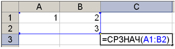
7_3: USE in Informatics 2016, "Typical test tasks in Informatics”, Krylova S.S., Churkina T.E. Option 2.:

A fragment of a spreadsheet is given.

From cell A3 into a cell C2
C2?

✍ Solution:

Result: 180

For an analysis of this 7 task, see the video:

7_4: USE in Informatics 2017, "Typical test tasks in Informatics", Krylova S.S., Churkina T.E. Option 5:

A3 into a cell E2 formula has been copied. When copying, the addresses of the cells have automatically changed.
What is the numeric value of the formula in the cell E2?

✍ Solution:

• Consider a formula in a cell A3:= $E$1*A2 . The dollar sign means absolute addressing: when you copy the formula, the letter or number next to the dollar will not change. That is, in our case, the factor $E$1 so it will remain in the formula when copying.
• Since copying is done in a cell E2, you need to calculate how many columns the formula will move to the right: 5 columns (from A before E). Accordingly, in the factor A2 letter A will be replaced by E.
• Now let's calculate how many lines the formula will move up when copying: one (c A 3 to E 2 ). Accordingly, in the factor A2 number 2 will be replaced by 1 .
• Get the formula and calculate the result: =$E$1*E1 = 1

Result: 1

7_5: 7 task. Demo version of the exam 2018 informatics:

A fragment of a spreadsheet is given. From cell B3 into a cell A4 formula has been copied. When copying the addresses of the cells in the formula, they automatically changed.
What is the numeric value of the formula in the cell A4?


Note: The $ sign denotes absolute addressing.

✍ Task 7 solution:

• The dollar sign $ means absolute addressing:
• The $ in front of the letter means the column is fixed: i.e. when copying the formula, the column name will not change;
• $ in front of the number means the line is fixed: when copying the formula, the name of the line will not change.
• In our case, the selected letters and numbers will not change: = $C 2+D $3
• Copying the formula one column to the left means that the letter D(in D$3) must change to the previous C. When copying the formula down one line, the value 2 (in $C2) changes to 3 .
• We get the formula:

= $C3 + C$3

As a result, we have the result: 300 + 300 = 600

Result: 600

For a detailed solution of this 7 task from the USE demo version of 2018, see the video:

What formula was written

7_6: 7 task of the exam. Task 6 GVE 11th grade 2018 (FIPI)

Kolya needs to build a table of formula values ​​using spreadsheets 5x–3y for values X and at from 2 before 5 . To do this, first in the ranges B1:E1 and A2:A5 he wrote down the numbers 2 before 5 . Then to cell IN 2 wrote down the formula (A2 - x value; B1 - y value), and then copied it to all cells of the range B2:E5. The result is the table below.


What formula was written in the cell IN 2?

Note: The $ sign is used to denote absolute addressing.

Options:
1)=5*$A$2–3*$B$1
2)=5*$A2–3*B$1
3)=5*A$2–3*$B1
4)=5*A2–3*$B$1

✍ Solution:

• Mentally imagine copying a cell with a formula separately horizontally and vertically.

Horizontally:

• Column reference in formula BUT should not change the letter when copying, which means that you must put a $ sign in front of it:

= 5 * $A

Whereas the column name B must change (to C, D, E) so that the numbers in the subtracted change (3, 4, 5):

= 3*B

Vertically:

The line number in the minuend must change so that the numbers in it increase (3, 4, 5). Whereas the lines in the subtrahend should not change: $A2. Thus, it is necessary to put a $ sign before the line number in the minuend: B$1

As a result, we get the formula: = 5 * $A2 - 3 * B$1, which corresponds to the number 2 .

Result: 2

Meaning of the SUM or AVERAGE formula

7_7: USE in computer science task 7 (example of task P-00, Polyakov K.)

Per

How the cell value will change C3, if after entering the formulas move the contents of the cell B2 in B3?
("+1" means an increase of 1 , "-one" means a decrease in 1 ):

Options:
1) -2
2) -1
3) 0
4) +1

✍ Solution:

Let's analyze the spreadsheet data before moving:
• In a cell C2 number will be 4 , since the function CHECK counts the number of nonblank cells in the specified range.
• In a cell C3 number will be 3 :

(1 + 2 + 2 + 6 + 4) / 5 = 3

Now let's see what happens after the move:

Moving the contents of a cell means that the cell B2 will be empty, and in the cell B3 a number will appear 6 .

Then the calculation of the formula in the cell C2 will change: the number of non-empty cells in the range A1:B2 becomes equal 3 .

The value will change accordingly after the calculation of the cell formula C3: the average value of the contents of a range of cells A1:C2 becomes equal to:

(1 + 2 + 2 + 3) / 4 = 2

(don't forget that the function AVERAGE does not take into account empty cells, so the cell B2 not taken into account).

Thus, the value after moving the formula has changed, decreasing by 1 . Correct answer 2

Result: 2

Detailed video solution:

7_8:

In the spreadsheet, the value of the formula =AVERAGE(C2:C5) is 3 .

What is the value of the formula =SUM(C2:C4) if the value of the cell C5 equals 5 ?

✍ Solution:

• Function AVERAGE is designed to calculate the arithmetic mean of the specified range of cells. Those. in our case, the average value of cells C2, C3, C4, C5.
• The result of the function =AVERAGE(C2:C5) is given by condition, let's substitute it into the formula:

(C2 + C3 + C4 + C5)/4 = 3

Let's take an unknown amount in x and get the formula for calculating the average value:

x / 4 = 3

Let's find x:

x = 3 * 4 = 12 -> C2 + C3 + C4 + C5 = 12

According to the assignment, you need to find = SUM (С2: С4) . Knowing the value in a cell C5, subtract it from the resulting sum and find the answer:

C2 + C3 + C4 = C2 + C3 + C4 + C5 -C5 = = 12 - 5 = 7

Result: 7

For a detailed solution, see the video:

What number should be in the cell

7_9: USE in Informatics 2017 assignment FIPI option 7 (Krylov S.S., Churkina T.E.):

Given a fragment of a spreadsheet:

A1 to have a chart based on cell values A2:C2 matched the picture? It is known that all cell values ​​from the considered range are non-negative.

✍ Solution:

• We have a pie chart that displays the shares of individual components in the total. From the image of the diagram, one can judge that, most likely, the values ​​in all cells of the formula should be equal (the sections of the diagram are visually equal).
• A1 -> x:

A2: x + 4 - 3 = x + 1 B2: (5 * x + 5) / 5 C2: (x + 1) * (x - 4) = x 2 - 3 * x - 4

Since the sectors of the diagram are equal, we equate any two of the resulting expressions (for example, C2 = A2):

x²-3 ​​* x - 4 = x + 1 x²-4 * x - 5 = 0 x1.2 = (4±√16 - 4 * 1 * (-5)) / 2 = (4±6) / 2 x1 = 5, x2 = -1

According to the condition of the assignment, the number should not be negative, so 5 suits us

Result: 5

For more detailed analysis we offer to watch the video of the solution of this 7 USE assignments in informatics:

Consider another example of solving task 7 of the exam in computer science:

7_10: USE in Informatics 2017 task 7 FIPI option 15 (Krylov S.S., Churkina T.E.):

Given a fragment of a spreadsheet:

What integer should be written in the cell C1 so that the chart built after performing the calculations by the values ​​of the range of cells A2:C2 did it match the picture?
It is known that all values ​​of the range on which the chart is built have the same sign.

✍ Solution:

• The pie chart displays the proportions of individual parts in the total. In our case, the chart reflects the results of calculating formulas in cells A2:C2
• From the diagram, one can judge that, most likely, the obtained values ​​in the formulas in all cells should be equal (the sectors of the diagram are visually equal).
• Get expressions from cell formulas by substituting C1 -> x:

A2: x + 2 B2: 8/2 = 4 C2: x * 2

Since the sectors of the diagram are equal, we equate two of the expressions obtained (for example, C2 = B2):

2 * x = 4 => x = 2

For this task you can get 1 point on the exam in 2020

Task 7 of the Unified State Examination in Informatics is devoted to the analysis of charts and spreadsheets. When solving this test, you will have to, for example, determine the values ​​of formulas by some parameters. A typical question of this option is: “If the arithmetic mean of four values ​​in the table is 5, then what is the sum of the first three cells, if the fourth cell contains the number 6, and there are no empty cells in the table.”

In other versions of task 7 of the Unified State Exam in computer science, the student will be asked to draw up a diagram based on the given data. For example, you are given the compositions of two substances with indications of the mass fractions of their components. It is required to determine the ratio of these elements in an alloy of two substances and find the correct one among the presented diagrams. Also, the ticket can contain tasks to determine the total income of each family member for some time, the volume of the harvest for each of the varieties of cucumbers, the number of schoolchildren participating in subjects in different regions of Russia, the increase in prices of some goods as a percentage relative to the beginning of the year .

Tasks of type A7 in informatics imply knowledge information processing technologies in spreadsheets. Even more specifically - absolute and relative addressing.

A7 Unified State Examination in Informatics

As an example, consider solution of problem A7 consider solution A7 of the demo version of the Unified State Examination 2013 in computer science:

A fragment of a spreadsheet is given.

	A	B	C	D
1	1	2	3
2	5	4	= $A$2 + B$3
3	6	7	= A3 + B3

What will the value of cell D1 become equal to if you copy the formula from
cells C2?
Note: The $ sign denotes absolute addressing.

1)18 2)12 3)14 4)17

Solution:

Let's look at the contents of cell C2. It contains a formula that uses two cells, and the cell references completely absolute($A$2) or partially absolute(B$3). When copying from cell C2 to cell D1, the address of cell $A$2 will remain the same, since its address is specified absolutely. The address of cell B$3 is set partially absolute - when copying, the row number will not change, but the column will change. When copying from column C to column D, the address of cell B$3 will change to 1 and become C$3. As a result, after copying, the formula = $A$2 + C$3 will appear in cell D1. We know the contents of cell A2 - it is equal to 5. The contents of cell C3 need to be calculated: A3 + B3 = 6 + 7 = 13. We get that the value of cell D1 will be 5 + 13 = 18. Correct answer 1.

As an anchor solve problem A7 of the demo version of the USE 2012 in computer science:

Cell B4 of the spreadsheet contains the formula = $C3*2. What will the formula look like when cell B4 is copied to cell B6?
Note: The $ sign is used to denote absolute addressing.

1) = $C5 *4 2) = $C5 *2 3) = $C3 *4 4) = $C1 *2

Solution:

In the formula = $C3 * 2, the addressing of cell $C3 is partially absolute - when copying, only the line number changes (because it is preceded by a $ sign), and the column will remain unchanged. When copying from cell B4 to cell B6, the row number will increase by 2, so the address of cell $C3 will become $C5. As a result, the formula = $C5 * 2 will be in cell B6. Correct answer 2.

7.1 (ege.yandex.ru-1) A fragment of a spreadsheet is given:

Solution:

From the second equation we find: С1=3. Let's check that this value is also suitable for the first equation:

2*(4-3) = 2*1 =2

Answer: 3

7.2 (ege.yandex.ru-2) A fragment of a spreadsheet is given:

What integer must be written in cell C1 in order for the pie chart built for the range A2:C2 to match the figure? It is known that all values ​​of the range on which the chart is built have the same sign.

Solution: The chart is based on the values ​​of three cells: A2, B2, C2. From the pie chart, you can see that these values ​​are related as 1:1:1. Since the values ​​of cells A1 and B1 are known, let's fill the range A2:C2 with values ​​instead of formulas (where possible):

Since the values ​​in all cells of the range A2:C2 must be equal, then for the value of C1 we obtain two equations:

From the second equation we find: С1=2. Let's check that this value is also suitable for the first equation:

Answer: 2

7.3 (ege.yandex.ru-3) A fragment of a spreadsheet is given:

What integer must be written in cell B1 so that the pie chart built for the range A2:C2 matches the picture? It is known that all values ​​of the range on which the chart is built have the same sign.

Solution 1: The chart is based on the values ​​of three cells: A2, B2, C2. From the pie chart, you can see that these values ​​are related as 2:1:1, while it is not known which cell corresponds to which sector of the chart. Let's simplify the formulas, given that we know the value for cell A1:

From the formula in cell C2, you can see that the values ​​for B2 and C2 are different. Therefore A2 = B2. This gives us the equation for B1:

3-B1 = (3*B1+3)/3

We solve the equation.

Answer: 1

Solution 2 (similar reasoning, a little shorter) : The chart is based on the values ​​of three cells: A2, B2, C2. From the pie chart, you can see that these values ​​are related as 2:1:1, while it is not known which cell corresponds to which sector of the chart. From the formula in cell C2, you can see that the values ​​for B2 and C2 are different. Therefore A2 = B2. Considering that C1 = A1+1 = 2+1 =3, we obtain the equation for B1

3-B1 = (3*B1+3)/3

We solve the equation.

Let's check ourselves - find the values ​​in all cells of the table

Answer: 1

7.4 (ege.yandex.ru-4) A fragment of a spreadsheet is given:

What integer must be written in cell A1 so that the pie chart built for the range A2:C2 matches the picture? It is known that all values ​​of the range on which the chart is built have the same sign.

Solution: The chart is based on the values ​​of three cells: A2, B2, C2. From the pie chart, you can see that these values ​​are related as X:1:1, where X is approximately equal to 4. It is not known which cell corresponds to which sector of the chart. Let's simplify the formulas in the table, given that C1=2. We get:

Since B2 > C2, A2=C2 must be satisfied. We get:

whence A1=7.

Answer: 7

7.5 (ege.yandex.ru-5) A fragment of a spreadsheet is given:

What integer must be written in cells B1 in order for the pie chart built for the range A2:C2 to match the figure? It is known that all values ​​of the range on which the chart is built have the same sign.

Solution: The chart is based on the values ​​of three cells: A2, B2, C2. From the pie chart, you can see that these values ​​are related as 2:1:1. That is, one of the values ​​(greater) is different from the others, and the two smaller values ​​are equal to each other. At the same time, it is not known which cell corresponds to which sector of the chart. Let's simplify the formulas in the table, given that A1=4. We get:

Let's look at the formula =B2+4 in cell C2. You can see that the value in cell C2 is 4 greater than the value in cell B2. In other words, the values ​​in cells B2 and C2 are different, while C2 > B2. So C2 is the larger of the three numbers, and A2 = B2 is the two smaller ones. At the same time, it can be seen from the diagram that C2 is twice as large as A2 and B2. Therefore done:

This gives us a system of two equations to determine the values ​​of B1 and C1:

B1-C1+4 = 2*(B1-C1)

From the 1st equation: B1 = 5*C1. We substitute into the 2nd equation:

5*C1 - C1 + 4 = 2*(5*C1-C1)

Therefore B1=5. We do a check - we calculate the values ​​​​for all cells: