Matrix addition.

Addition properties:

· A + B = B + A.

· (A + B) + C = A + (B + C).

Multiplying a matrix by a number.

· k(A + B) = kA + kB.

· (k + m)A = kA + mA.

Matrix multiplication.

Inverse matrix.

Properties of determinants

4. Substitution theorem.

5. Cancellation theorem.

additions to these elements

where i= ,

Transposing matrices.

Transposed matrix
A T [ i, j] = A[j, i].
For example,

And

Cylindrical surfaces.

A surface formed by the movement of a straight line L, which moves in space, maintaining a constant direction and intersecting each time a certain curve K, is called a cylindrical surface or cylinder; curve K is the guide of the cylinder, and L is its generator.

Elliptical cylinder

Elliptic equation:

A special case elliptical cylinder is circular cylinder, its equation is x 2 + y 2 = R 2 . The equation x 2 =2pz defines in space parabolic cylinder.

The equation: defines in space hyperbolic cylinder.

All these surfaces are called second order cylinders, since their equations are equations of the second degree with respect to the current coordinates x, y, z.

62. Ellipsoids.

Let us examine the surface defined by the equation:

Let us consider sections of a surface with planes parallel to the xOy plane. Equations of such planes: z=h, where h is any number. The line obtained in the section is determined by two equations:

Let's examine the surface:

And if That The line of intersection of the surface with the z=h planes does not exist.

B) if , the intersection line degenerates into two points (0,0,c), and (0,0,-c). The plane z = c, z = - c touches the given surface.

B) if , then the equations can be rewritten as:
, as can be seen, the intersection line is an ellipse with semi-axes a1 = , b1 = . In this case, the smaller h, the larger the semi-axes. At n=0 they reach their highest values: a1=a, b1=b. The equations will take the form:

The sections considered make it possible to depict the surface as a closed oval surface. The surface is called an ellipsoid. If any semi-axes are equal, the triaxial ellipsoid turns into an ellipsoid of revolution, and if a=b=c, then into a sphere.

Hyperboloids.

1. Examine the surface . Intersecting the surface with the plane z=h, we obtain an intersection line whose equations have the form

z=h. or z=hsemi-axis: a1= b1=

the semi-axes reach their minimum value at h=0: a1=a, b1=b. As h increases, the semi-axes of the ellipse will increase. => x=0.

Analysis of these sections shows that the surface defined by the equation has the shape of an infinite expanding tube. The surface is called single-sheet hyperboloid.

2. - surface equation.

And - a surface consisting of 2 cavities shaped like convex unlimited bowls. The surface is called two-sheet hyperboloid.

64. paraboloids.

.
-This elliptical paraboloid.

Canonical equation: (p>0, q>0).

p = q is a paraboloid of rotation around the Oz axis.

Sections of an elliptic paraboloid by planes are either an ellipse, a parabola, or a point.

2.
- hyperbolic paraboloid.

Sections of a hyperbolic paraboloid by planes are either a hyperbola, a parabola, or a pair of straight lines (rectilinear generators).

65. Canonical surfaces.

Canonical equation:

a = b - cone of rotation (straight circular)
Sections of a cone by planes: in the plane intersecting all rectilinear generatrices - an ellipse; in a plane parallel to one rectilinear generatrix - a parabola; in a plane parallel to two rectilinear generators - a hyperbola; in the plane passing through the vertex of the cone - a pair of intersecting lines or a point (vertex).

66. Function. Basic concepts. Ways to set it.

A function is a law according to which a number x from a given set X is associated with only one number y, written , while x is called the argument of the function, y

called the value of the function.

1. Analytical method.

2. Graphic method.

3. Verbal method.

4. Tabular method.

Comparison theorem.

in the theory of differential equations, a theorem stating the presence of a certain property of solutions to a differential equation (or system of differential equations) under the assumption that an auxiliary equation or inequality (system of differential equations or inequalities) has some property.

1) Sturm’s theorem: any nontrivial solution to the equation vanishes on the interval no more than m times if the equation and for has this property.

2) Differential inequality: the solution to the problem is component-wise non-negative if the solution to the problem has this property and the inequalities are satisfied

The first is a wonderful limit.

When calculating the limits of expressions containing trigonometric functions, the limit is often used called the first remarkable limit.

It reads: the limit of the ratio of a sine to its argument is equal to one when the argument tends to zero.

Proof:

Let's take a circle of radius 1 and denote the radian measure of the angle MOV by x. let 0 , arc MV is numerically equal to the central angle x, . Obviously, we have . Based on the corresponding geometry formulas, we obtain . Let's divide the inequality by >0, We get 1<

Because , then based on the criterion (on the limit of an intermediate function) of the existence of limits .

And if x<0 => , where –x>0 =>

83. The second remarkable limit.

As is known, the limit of a number sequence
, has a limit equal to e. . 1.Let . Each x value is enclosed between two positive integers: , where n=[x] is the integer part of x. It follows that therefore
. If , That . That's why:
,

Based on the existence of limits: . 2. Let . Let's make the substitution –x=t, then = . And called the second remarkable limit. They are widely used in calculating limits. In analytical applications, the exponential function with base e plays an important role. Function is called exponential, the notation is also used .

Proof.

(taking into account that if Dx®0, then Du®0, since u = g(x) is a continuous function)

Then . The theorem has been proven.

Cauchy's theorem

Cauchy's theorem: If the functions f(x) and are continuous on the interval, differentiable on the interval (a,b), and For , then there is at least one point , such that the equality
.

Matrices. Basic concepts. Linear operations on matrices and their properties.

A matrix of size m by n is a collection of mn real (complex) numbers or elements of another structure (polynomials, functions, etc.), written in the form of a rectangular table, which consists of m rows and n columns and taken into round or rectangular or double straight brackets. In this case, the numbers themselves are called matrix elements and each element is associated with two numbers - the row number and the column number.

A matrix whose elements are all zero is called a zero matrix

A matrix of size n by n is called a square matrix of nth order, i.e. the number of rows is equal to the number of columns.

A square matrix is ​​called diagonal if all its off-diagonal elements are zero.

A diagonal matrix in which all diagonal elements are equal to 1 is called the identity matrix
Matrix addition.

Addition properties:

· A + B = B + A.

· (A + B) + C = A + (B + C).

· If O is a zero matrix, then A + O = O + A = A

Remark 1. The validity of these properties follows from the definition of the operation of matrix addition.

Remark 2. Note again that only matrices of the same dimension can be added.

Multiplying a matrix by a number.

Properties of multiplying a matrix by a number

· k(A + B) = kA + kB.

· (k + m)A = kA + mA.

Remark 1. The validity of the properties follows from Definitions 3.4 and 3.5.

Remark 2. Let us call the difference of matrices A and B a matrix C for which C+B=A, i.e. C=A+(-1)B.
Matrix multiplication.

Multiplying a matrix by a matrix also requires certain conditions to be met for the dimensions of the factors, namely: the number of columns of the first factor must be equal to the number of rows of the second.

For square matrices of the same order, the products AB and BA exist and have the same dimension, but their corresponding elements are generally not equal.

However, in some cases the products AB and BA coincide

Inverse matrix.

A square matrix A is called singular if ∆A=0, and non-singular if ∆A≠0

A square matrix B is called the inverse of a square matrix A of the same order if AB = BA = E. In this case, B is denoted

For an inverse matrix to exist, it is necessary and sufficient that the original matrix be nonsingular.

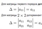
2. Matrix determinant. Properties of determinants.

Determinant (or determinant) is one of the basic concepts of linear algebra. The determinant of a matrix is ​​a polynomial of the elements of a square matrix (that is, one in which the number of rows and columns is equal). In general, a matrix can be defined over any commutative ring, in which case the determinant will be an element of the same ring. (∆A)

Properties of determinants

· The determinant is a skew-symmetric polylinear function of the rows (columns) of the matrix. Multilinearity means that the determinant is linear over all rows (columns): , where, etc. are the rows of the matrix, is the determinant of such a matrix.

· When adding a linear combination of other rows (columns) to any row (column), the determinant will not change.

· If two rows (columns) of a matrix coincide, then its determinant is zero.

· If two (or several) rows (columns) of a matrix are linearly dependent, then its determinant is equal to zero.

· If you rearrange two rows (columns) of a matrix, then its determinant is multiplied by (-1).

· The common factor of the elements of any series of the determinant can be taken out of the sign of the determinant.

· If at least one row (column) of the matrix is ​​zero, then the determinant is equal to zero.

· The sum of the products of all elements of any row by their algebraic complements is equal to the determinant.

· The sum of the products of all elements of any series by the algebraic complements of the corresponding elements of a parallel series is zero.

· The determinant of the product of square matrices of the same order is equal to the product of their determinants (see also the Binet-Cauchy formula).

· Using index notation, the determinant of a 3x3 matrix can be determined using the Levi-Civita symbol from the relation:

3. Minors and algebraic complements.

The minor of an nth order matrix element is the determinant of a (n-1)th order matrix obtained from matrix A by deleting the i-th row and j-th column.

When writing out the determinant of the (n-1)th order, in the original determinant the elements located under the lines are not taken into account.
The algebraic complement Aij of an element aij of an nth order matrix is ​​its minor, taken with a sign, depending on the row number and column number: that is, the algebraic complement coincides with the minor when the sum of the row and column numbers is an even number, and differs from the minor in sign, when the sum of the row and column numbers is an odd number.

4. Substitution theorem.

The sums of the products of arbitrary numbers bi ,b2,...,b by the algebraic complements of the elements of any column or row of a matrix of order n are equal to the determinant of the matrix, which is obtained from this by replacing the elements of this column (row) with the numbers b1,b2,...,bn.

5. Cancellation theorem.

The sum of the products of the elements of one of the columns (rows) of the matrix by the corresponding algebraic complements of the elements of another column (row) is equal to zero.

6. Some methods for calculating determinants.

Theorem (Laplace). Determinant of a matrix of order N = the sum of the product of all minors of kth order, which can be composed of arbitrarily chosen k parallel series and algebraic complements of these minors

Theorem (on the expansion of the determinant into elements of a series). Qualifier sq. matrix = the sum of products of elements of a certain series and algebraic

additions to these elements

7. Matrix multiplication. Properties of multiplication.

The operation of multiplying two matrices is introduced only for the case when the number of columns of the first matrix is ​​equal to the number of rows of the second matrix.

The product of matrix A m * n = (a i , g) by matrix B n * p = (b i , k) is a matrix Cm*p = (with i , k) such that: ,

where i= , , i.e. the element of the i-th and k-th columns of the product matrix C is equal to the sum of the products of the elements of the i-th row of matrix A with the corresponding elements of the k-th column of matrix B.

Matrices A, n*m and B, m*n, called. agreed upon. (if A is consistent with B, this does not mean that B is consistent with A).

The meaning of consistency is that the number of columns of the 1st matrix coincides with the number of rows of the 2nd matrix. For matched matrices, a multiplication operation can be defined.

If matrices A and B are square and of the same size, then A*B and B*A always exist. Transposition is the change of all elements of a column to the corresponding elements of a row. If A T =A, then the matrix A is called. symmetrical (it must be square).

Transposing matrices.

Transposed matrix- matrix obtained from the original matrix by replacing rows with columns.
Formally, the transposed matrix for a size matrix is ​​a size matrix, defined as A T [ i, j] = A[j, i].
For example,

And

Inverse matrix. A necessary and sufficient condition for the existence of an inverse matrix. Finding the inverse matrix.

Let there be a matrix A - non-singular.

A -1 , A -1 *A=A*A -1 =E, where E is the identity matrix. A -1 has the same dimensions as A.

Algorithm for finding the inverse matrix:

1. Instead of each element of the matrix a ij, we write its algebraic complement.

A* is a union matrix.

2. transpose the resulting union matrix. A * T

3. divide each element of the union matrix by the determinant of matrix A.

A -1 = A *T

Theorem: (about the cancellation of the determinant):
the sum of the products of elements of a certain series of a determinant by the algebraic complement to the elements of another parallel series is always equal to zero.

10. Matrix representation of a system of linear equations and its solutions.

Matrices make it possible to briefly write down a system of linear equations. Let a system of 3 equations with three unknowns be given:

Consider the system matrix and matrices columns of unknown and free terms

Let's find the work

those. as a result of the product, we obtain the left-hand sides of the equations of this system. Then, using the definition of matrix equality, this system can be written in the form

or shorter A∙X=B.

Here are the matrices A And B are known, and the matrix X unknown. It is necessary to find it, because... its elements are the solution to this system. This equation is called matrix equation.

Let the matrix determinant be different from zero | A| ≠ 0. Then the matrix equation is solved as follows. Multiply both sides of the equation on the left by the matrix A-1, inverse of the matrix A: . Because the A -1 A = E And E∙X = X, then we obtain a solution to the matrix equation in the form X = A -1 B.

Note that since the inverse matrix can only be found for square matrices, the matrix method can only solve those systems in which the number of equations coincides with the number of unknowns. However, matrix recording of the system is also possible in the case when the number of equations is not equal to the number of unknowns, then the matrix A will not be square and therefore it is impossible to find a solution to the system in the form X = A -1 B.

11. Solution of non-degenerate linear systems, Cramer formulas.

It is customary to write SLAEs in matrix form, when the unknowns themselves are not indicated, but only the matrix of system A and the column of free terms B are indicated.

Solving non-degenerate SLAEs using Cramer's method:

A -1 =

X1= (A 11 b 1 + A 21 b 2 + …+A n 1 b n)

Theorem: (Cramer):
solution of non-degenerate equations AX=B, can be written like this:

, Ak is obtained from A by replacing the k-th column with the column of the free term B.

12. Matrix rank. Properties of matrix rank. Calculating the rank of a matrix using elementary transformations.

The maximum number of linearly dependent rows of the matrix A is called. rank of the matrix and denotation r(a). The largest of the minor orders of a given matrix other than 0 is called matrix rank.

Properties:

1) when transposing rank=const.

2) if you cross out the zero row, then rang=const;

3)rang=cost, with elementary transformations.

3) to calculate the rank using the element, transform matrix A into matrix B, the rank of which is easily found.

4) rank of matrix triangle = number of non-zero elements located on the main diagonals.

Methods for finding the rank of a matrix:

1) method of bordering minors

2) method of elementary transformations

Bordering minors method:

The method of bordering minors allows you to algorithmize the process of finding the rank matrix and allows you to minimize the number of calculations of minors.

1) if the matrix has all zero elements, then rank = 0

2) if there is at least one non-zero element => r(a)>0

Now we will border the minor M1, i.e. we will construct all possible minors of the 2nd order, ktr. contain the i-th row and the j-th column until we find a non-zero minor of the 2nd order.

The process will continue until one of the following events occurs:
1. The size of the minor will reach the number k.

2. at some stage all bordered minors will turn out to be = 0.

In both cases, the magnitude of the rank matrix will be equal to the order of the larger non-zero minor.

Elementary transformation method:
As is known, the concept of a triangular matrix is ​​defined only for square matrices. For rectangular matrices, an analogue is the concept of a trapezoidal matrix.

For example:
rank = 2.

For each numbers a¹0 there is an inverse number a -1 such that the work a×a -1 =1. A similar concept is introduced for square matrices.

Definition. If there are square matrices X and A of the same order satisfying the condition:

where E is the identity matrix of the same order as the matrix A, then the matrix X is called reverse to the matrix A and is denoted by A -1.

From the definition it follows that only a square matrix has an inverse; in this case, the inverse matrix is ​​also square of the same order.

However, not every square matrix has an inverse. If the condition a¹0 is necessary and sufficient for the existence of a number a -1, then for the existence of matrix A -1 such a condition is the requirement DA ¹0.

Definition. Square matrix n-th order is called non-degenerate (non-singular), if its determinant is DA ¹0.

If DA= 0 , then matrix A is called degenerate (special).

Theorem(a necessary and sufficient condition for the existence of an inverse matrix). If a square matrix not special(i.e. its determinant is not equal to zero), then for it there exists the only one inverse matrix.

Proof.

I. Necessity. Let matrix A have an inverse A -1, i.e. AA -1 = A -1 A=E. By property 3 determinants ( § 11) we have D(AA -1)= D(A -1) D(A)= D(E)=1, i.e. D.A. ¹0 and DA -1 ¹0.

I I. Adequacy. Let the square matrix A be non-singular, i.e. D.A. ¹0 . Let's write the transposed matrix A T:

In this matrix, we replace each element with its algebraic complement, and we obtain the matrix:

The matrix A* is called annexed matrix to matrix A.

Let's find the product AA * (and A * A):

Where diagonal elements = DA,

DA.(formula 11.1 §eleven)

And everyone else off-diagonal elements of matrix AA * are equal to zero property 10 §11, For example:

etc. Hence,

AA * = or AA * = DA= DA×E.

Similarly, it is proved that A * A = DA×E.

Dividing both obtained equalities by DA, we get: . This, by the definition of an inverse matrix, implies the existence of an inverse matrix

Because AA -1 =A -1 A=E.

The existence of an inverse matrix has been proven. Let's prove uniqueness. Suppose that there is another inverse matrix F for matrix A, then AF = E and FA = E. Multiplying both sides of the first equality by A -1 on the left, and the second by A -1 on the right, we get: A -1 AF = A - 1 E and FA A -1 = E A -1, whence EF = A -1 E and FE = E A -1. Therefore, F = A -1. Uniqueness has been proven.

Example. Given a matrix A = , find A -1 .

Algorithm for calculating the inverse matrix:

Properties of inverse matrices.

1) (A -1) -1 = A;

2) (AB) -1 = B -1 A -1

3) (A T) -1 = (A -1) T .

⇐ Previous78910111213141516Next ⇒

⇐ PreviousPage 3 of 4Next ⇒

Let's consider the matrices

Moreover, the elements of matrices A and B are given, and X 1, X 2, X 3 are unknown.

Then the equation A × X = B is called the simplest matrix equation.

To solve it, i.e. to find the elements of the matrix of unknowns X, we proceed as follows:

1. Multiply both sides of the equation by matrix A -1, the inverse of matrix A , left:

A -1 (A × X) = A -1 × B

2. Using the property of matrix multiplication, we write

(A -1 × A) X = A -1 × B

3. From the definition of an inverse matrix

(A -1 × A = E) we have E × X = A -1 × B.

4. Using the property of the identity matrix (E × X = X), we finally obtain X = A -1 × B

Comment. If the matrix equation has the form X × C = D, then to find the unknown matrix X the equation must be multiplied by C -1 on right.

Example. Solve matrix equation

Solution. Let us introduce the notation

Their definition of matrix multiplication, taking into account dimensions A and B, the matrix of unknowns X will have the form

Taking into account the introduced notation we have

A × X = B whence X = A -1 × B

Let's find A -1 using the algorithm for constructing the inverse matrix

Let's calculate the product

Then for X we get

X = whence x 1 = 3, x 2 = 2

Matrix rank

Consider a matrix A of size (m x n)

The kth order minor of a matrix A is the determinant of order k, the elements of which are the elements of the matrix A that stand at the intersection of any K rows and any K columns. Obviously, k £ min (m, n).

Definition. The rank r(A) of a matrix A is the highest order of the non-zero minor of this matrix.

Definition. Any nonzero minor of a matrix whose order is equal to its rank is called basic minor.

Define e. Matrices having the same ranks are called equivalent.

Calculating Matrix Rank

Definition. The matrix is ​​called stepped, if the first non-zero element of each row contains zeros in the underlying rows.

Theorem. The rank of an echelon matrix is ​​equal to the number of its nonzero rows.

Thus, by transforming the matrix into echelon form, it is easy to determine its rank. This operation is carried out using elementary matrix transformations, which do not change its rank:

— multiplication of all elements of the matrix row by the number l ¹ 0;

- replacing rows with columns and vice versa;

— rearrangement of parallel rows;

— crossing out the zero row;

- adding to the elements of a certain series the corresponding elements of a parallel series, multiplied by any real number.

Example.

Theorem (necessary and sufficient condition for the existence of an inverse matrix).

Calculate matrix rank

A =

Solution. Let's transform the matrix to echelon form. To do this, add the second line to the third line, multiplied by (-3).

A~

Let's add a third to the fourth line.

The number of non-zero rows in the resulting equivalent matrix is ​​three, therefore r(A) = 3.

Systems of n linear equations with n unknowns.

Methods for solving them

Consider a system of n linear equations with n unknowns.

A 11 x 1 + a 12 x 2 + ... + a 1 n x n = b 1

a 21 x 1 + a 22 x 2 + ... + a 2 n x n = b 2 (1)

……………………………….

a n 1 x 1 + a n 2 x 2 + … + a nn x n = b n

Definition: The solution to system (1) is a set of numbers (x 1, x 2, ..., x n), which turns each equation of the system into a true equality.

Matrix A, composed of coefficients for unknowns, is called main matrix of the system (1).

A=

Matrix B, consisting of elements of matrix A and a column of free terms of system (1), is called extended matrix.

B =

Matrix method

Let's consider the matrices

X = — matrix of unknowns;

С = is the matrix of free terms of system (1).

Then, according to the rule of matrix multiplication, system (1) can be represented as a matrix equation

A × X = C (2)

The solution to equation (2) is stated above, that is, X = A -1 × C, where A -1 is the inverse matrix for the main matrix of system (1).

Cramer method

A system of n linear equations with n unknowns, the main determinant of which is nonzero, always has a solution and, moreover, a unique one, which is found according to the formulas:

where D = det A is the determinant of the main matrix A of system (1), which is called the main one, Dх i are obtained from the determinant D by replacing the i-th column with a column of free terms, i.e.

Dx 1 = ;

Dx 2 = ; … ;

Example.

Solve a system of equations using Cramer's method

2x 1 + 3x 2 + 4x 3 = 15

x 1 + x 2 + 5x 3 = 16

3x 1 - 2x 2 + x 3 = 1

Solution.

Let us calculate the determinant of the main matrix of the system

D = det A = = 44 ¹ 0

Let's calculate auxiliary determinants

Dx 3 = = 132.

Using Cramer's formulas we will find the unknowns

; ; .

Thus x 1 = 0; x 2 = 1; x 3 = 3.

Gauss method

The essence of the Gauss method is the sequential elimination of unknowns from the equations of the system, i.e. in reducing the main matrix of the system to a triangular form, when there are zeros under its main diagonal. This is achieved using elementary matrix transformations over the rows. As a result of such transformations, the equivalence of the system is not violated and it also acquires a triangular shape, i.e. the last equation contains one unknown, the penultimate two, etc. Expressing the nth unknown from the last equation and using the reverse motion, using a series of successive substitutions, the values ​​of all unknowns are obtained.

Example. Solve a system of equations using the Gauss method

3x 1 + 2x 2 + x 3 = 17

2x 1 - x 2 + 2x 3 = 8

x 1 + 4x 2 - 3x 3 = 9

Solution. Let us write down the extended matrix of the system and reduce the matrix A contained in it to a triangular form.

Let's swap the first and third rows of the matrix, which is equivalent to rearranging the first and third equations of the system. This will allow us to avoid the appearance of fractional expressions in subsequent calculations

B~

We multiply the first row of the resulting matrix sequentially by (-2) and (-3) and add it with the second and third rows, respectively, and B will have the form:

After multiplying the second row by and adding it to the third row, matrix A will take on a triangular form. However, to simplify the calculations, you can do the following: multiply the third line by (-1) and add it to the second. Then we get:

B~

B~

Let us restore from the resulting matrix B a system of equations equivalent to this

X 1 + 4x 2 - 3x 3 = 9

x 2 - 2x 3 = 0

— 10x 3 = -10

From the last equation we find We substitute the found value x 3 = 1 into the second equation of the system, from which x 2 = 2x 3 = 2 × 1 = 2.

After substituting x 3 = 1 and x 2 = 2 into the first equation for x 1, we get x 1 = 9 - 4x 2 + 3x 3 = 9 - 4 × 2 + 3 × 1 = 4.

So x 1 = 4, x 2 = 2, x 3 = 1.

Comment. To check the correctness of the solution of a system of equations, it is necessary to substitute the found values ​​of the unknowns into each of the equations of this system. Moreover, if all equations turn into identities, then the system is solved correctly.

Examination:

3 × 4 + 2 × 2 + 1 = 17 correct

2 × 4 – 2 + 2 × 1 = 8 correct

4 + 4 × 2 – 3 × 1 = 9 correct

So, the system is solved correctly.

⇐ Previous1234Next ⇒

Read also:

The simplest matrix equations

where are matrices of such sizes that all the operations used are possible, and the left and right sides of these matrix equations are matrices of the same size.

The solution of equations (1)-(3) is possible using inverse matrices in the case of non-degenerate matrices for X. In the general case, the matrix X is written element-by-element and the actions specified in the equation are performed on the matrices. As a result, a system of linear equations is obtained. Having solved the system, find the elements of the matrix X.

Inverse matrix method

This is a solution to a system of linear equations in the case of a square non-singular matrix of system A. It is found from the matrix equation AX=B.

A -1 (AX)=A -1 V, (A -1 A)X=A -1 V, EX= A -1 V, X= A -1 V.

Cramer's formulas

Theorem.Let Δ — is the determinant of the matrix of system A, and Δ j is the determinant of the matrix obtained from matrix A by replacing the jth column of free terms. Then, if Δ≠ 0, then the system has a unique solution, determined by the formulas:

- Cramer's formulas.

DZ 1. 2.23, 2.27, 2.51,2.55, 2.62; DZ 2.2.19, 2.26, 2.40,2.65

Topic 4. Complex numbers and polynomials

Complex numbers and operations on them

Definitions.

1. We will agree to call a symbol of the form a + bi, where a and b are arbitrary real numbers, a complex number.

2. We agree to consider complex numbers a + bi and a 1 + b 1 i equal if a = a 1 and

b = b 1 .

3. We agree to consider a complex number of the form a + 0i equal to the real number a.

4. The sum of two complex numbers a + bi and a 1 + b 1 i is called the complex number (a + a 1) + (b + b 1)i.

Inverse matrix. Matrix rank.

The product of two complex numbers is the complex number aa 1 – bb 1 + (a b 1 +a 1 b)i.

Complex number of the form 0 + bi is called a purely imaginary number and is usually written like this: bi; number 0 +1 i = i called imaginary unit.

By Definition 3, every real number A corresponds to an “equal” complex number a+0i and vice versa - to any complex number a+0i corresponds to an "equal" real number A, that is, there is a one-to-one correspondence between these numbers. If we consider the sum and product of complex numbers a 1 + 0i and a 2 + 0i according to rules 4 and 5, we get:

(a 1 + 0i) + (a 2 + 0i) = (a 1 + a 2) + 0i,

(a 1 + 0i) (a 2 + 0i) = (a 1 a 2 – 0) + (a 1 0+a 2 0) i = a 1 a 2 + 0i.

We see that the sum (or product) of these complex numbers corresponds to a real number “equal” to the sum (or product) of the corresponding real numbers. So, the correspondence between complex numbers of the form a+0i and real number A is such that as a result of performing arithmetic operations on the corresponding components, corresponding results are obtained. A one-to-one correspondence that is maintained when performing actions is called isomorphism. This allows us to identify the number a+0i with real number A and consider every real number as a special case of a complex number.

Consequence. Number square i equals – 1.

i 2 = i i = (0 +1i)(0 +1i) = (0 – 1) + (0 1 + 1 0)i =— 1.

Theorem.For addition and multiplication of complex numbers, the basic laws of operation remain in force.

Definitions:

1. The real number a is called the real part of the complex number z = a + bi. Rez=a

2. The number b is called the imaginary part of the complex number z, the number b is called the coefficient of the imaginary part of z. Imz=b.

3. The numbers a + bi and a – bi are called conjugate.

Conjugate number z = a + bi indicated by the symbol

= a - bi.

Example. z =3 + i,= 3 - i.

Theorem.The sum and product of two conjugate complex numbers are real.

Proof. We have

In the set of complex numbers, the inverse of addition and multiplication can be performed.

Subtraction. Let z 1 = a 1 + b 1 i And z 2 = a 2 + b 2 i are complex numbers. difference z 1 – z 2 there is a number z = x + yi, satisfying the condition z 1 = z 2 + z or

a 1 + b 1 i = (a 2 + x) + (b 2 + y)i.

For determining x And y we get a system of equations a 2 + x = a 1 And b 2 + y = b 1, which has a unique solution:

x = a 1 - a 2, y = b 1 - b 2,

z = (a 1 + b 1 i) – (a 2 + b 2 i) = a 1 – a 2 + (b 1 – b 2)i.

Subtraction can be replaced by addition with the opposite number of the one being subtracted:

z = (a 1 + b 1 i) – (a 2 + b 2 i) = (a 1 + b 1 i) + (- a 2 – b 2 i).

Division.

Quotient of numbers z 1 And z 2≠ 0 is a number z = x + yi, satisfying the condition z 1 = z 2 z or

a 1 + b 1 i = (a 2 + b 2 i) (x + yi),

hence,

a 1 + b 1 i = a 2 x - b 2 y+ (b 2 x + a 2 y)i,

from where we get the system of equations:

a 2 x - b 2 y = a 1 ,

b 2 x + a 2 y = b 1 .

The solution to which will be

hence,

In practice, to find the quotient, multiply the dividend and the divisor by the conjugate of the divisor:

For example,

In particular, the inverse of a given number z, can be represented in the form

Note. In the set of complex numbers remains valid theorem: if the product is equal to zero, then at least one of the factors is equal to zero.

In fact, if z 1 z 2 =0 and if z 1 ≠ 0, then multiplying by , we get

Q.E.D.

When performing arithmetic operations on complex numbers, you should be guided by the following general rule: actions are performed according to the usual rules for actions on algebraic expressions, followed by replacing i 2 with-1.

Theorem.When each component is replaced by its conjugate number, the result of the action is also replaced by its conjugate number.

The proof lies in direct verification. So, for example, if each term z 1 = a 1 + b 1 i And z 2 = a 2 + b 2 i replace with the conjugate number, we get the conjugate of the sum z 1 + z 2 .

therefore,

Similarly for the product we have:

Previous567891011121314151617181920Next

SEE MORE:

Matrix equations

Katalin David

AX = B, where matrix A is invertible

Since matrix multiplication is not always commutative, we multiply both sides of the equation from the left by $ A^(-1) $.

$A^(-1)\cdot|A\cdot X = B$

$A^(-1)\cdot A\cdot X = A^(-1)\cdot B$

$I_(n)\cdot X = A^(-1)\cdot B$

$\color(red)(X =A^(-1)\cdot B)$

Example 50
Solve the equation
$\begin(pmatrix) 1 & 3\\ 2 & 5 \end(pmatrix)\cdot X \begin(pmatrix) 3 & 5\\ 2 & 1 \end(pmatrix)$

Theorem 2. Criterion for the existence of an inverse matrix.

We multiply from the left by its inverse matrix.
$\begin(pmatrix) 1 & 3\\ 2 & 5\\ \end(pmatrix)^(-1)\cdot \begin(pmatrix) 1 & 3\\ 2 & 5 \end(pmatrix)\cdot X= \begin(pmatrix) 1 & 3\\ 2 & 5 \end(pmatrix)^(-1)\cdot \begin(pmatrix) 3 & 5\\ 2 & 1 \end(pmatrix)$

$I_(2)\cdot X = \begin(pmatrix) 1 & 3\\ 2 & 5 \end(pmatrix)^(-1)\cdot \begin(pmatrix) 3 & 5\\ 2 & 1 \end( pmatrix)$

$X=\begin(pmatrix) 1 & 3\\ 2 & 5 \end(pmatrix)^(-1)\cdot \begin(pmatrix) 3 & 5\\ 2 & 1 \end(pmatrix)$

$\begin(pmatrix) 1 & 3\\ 2 & 5 \end(pmatrix)^(-1)= \begin(pmatrix) -5 & 3\\ 2 & -1 \end(pmatrix)\rightarrow X= \ begin(pmatrix) -5 & 3\\ 2 & -1 \end(pmatrix)\cdot \begin(pmatrix) 3 & 5\\ 2 & 1 \end(pmatrix)= \begin(pmatrix) -9 & -22 \\ 4 & 9 \end(pmatrix)$

XA = B, where matrix A is invertible

Since matrix multiplication is not always commutative, we multiply both sides of the equation on the right by $ A^(-1) $.

$X\cdot A = B |\cdot A^(-1)$

$X\cdot A\cdot A^(-1) = B\cdot A^(-1)$

$X \cdot I_(n) =B\cdot A^(-1)$

The solution to the equation has the general form
$\color(red)(X =B\cdot A^(-1))$

Example 51
Solve the equation
$X \begin(pmatrix) 1 & 3\\ 2 & 5\\ \end(pmatrix)= \begin(pmatrix) 3 & 5\\ 2 & 1\\ \end(pmatrix)$

Let's make sure that the first matrix is ​​invertible.
$\left|A\right|=5-6=-1\neq 0$, therefore, the matrix is ​​invertible.

We multiply on the right by its inverse matrix.
$X \begin(pmatrix) 1 & 3\\ 2 & 5 \end(pmatrix)\cdot \begin(pmatrix) 1 & 3\\ 2 & 5 \end(pmatrix)^(-1)= \begin(pmatrix ) 3 & 5\\ 2 & 1 \end(pmatrix)\cdot \begin(pmatrix) 1 & 3\\ 2 & 5 \end(pmatrix)^(-1)$

$X\cdot I_(2)= \begin(pmatrix) 3 & 5\\ 2 & 1 \end(pmatrix)\cdot \begin(pmatrix) 1 & 3\\ 2 & 5 \end(pmatrix)^(- 1)$

$X=\begin(pmatrix) 3 & 5\\ 2 & 1 \end(pmatrix)\cdot \begin(pmatrix) 1 & 3\\ 2 & 5 \end(pmatrix)^(-1)$

$\begin(pmatrix) 1 & 3\\ 2 & 5 \end(pmatrix)^(-1)= \begin(pmatrix) -5 & 3\\ 2 & -1 \end(pmatrix)\rightarrow X= \ begin(pmatrix) 3 & 5\\ 2 & 1 \end(pmatrix) \cdot \begin(pmatrix) -5 & 3\\ 2 & -1 \end(pmatrix)= \begin(pmatrix) -5 & 4\ \ -8 & 5 \end(pmatrix)$

MatricesMatrix multiplicationDeterminantsMatrix rankInverse matricesSystems of equationsCalculators for matrices

intl. amazement, surprise; joy, hope; suddenness, fright; grief, despair. Oh, how good! Oh, if only it were so! Oh, how you scared me! Oh, and wave your hands. Oh, oh, but there’s nothing to help with. Ah, judge, judge: four skirts, eight pockets.

| Sometimes ah turns into a noun. , husband. Ahhs, ohhs, and women's sighs. What was there about gasps, surprise, joy. Ahti, ahhli to me, an exclamation of grief, sadness; Alas; I’m so excited, all my comrades are in prison - will there be something for me too? Ohti-axmul somehow get married? Not so hot for me, not amazing, not too good. Ahkhanki to me, akhanki, expresses, as it were, compassion for oneself or for another. Oh, like little children, this is a kind of greeting. Gasp, gasp, gasp, marvel; rejoice at something, grieve, moan, exclaim ah! I wish I was at home, on my own. Uncle would gasp, looking at himself, take care of yourself, about your business. I gasped, I was scared, I was amazed. We also gasped and saw grief. A single man will sometimes groan, and a married man will gasp.

inverse matrix

What the heck. We gasped when we learned about this. Let's go, let's go. I was amazed at these miracles. They gasped, or what? Cheer some more. One gasps, the other gasps. Why did you get excited? You will groan involuntarily. You gasp wrong, gasp again, a mockery of useless cries. I spent the whole day groaning. The woman came to gasp, but had to gasp; I came to look at someone else’s joy or sorrow, but my own misfortune happened. Aah Wed. immoderate expression of joy, amazement, grief, despair: gasping husband. ahalschnitsa no. gasped about. whoever marvels at everything, praises other people's things beyond measure, is envious. There are seven achalers for each achaler. For each bakhar there are seven ahals. Akhova lower Akhtitelny Penz. delightful, incredibly beautiful, beautiful, causing an exclamation of amazement and approval. Awful handkerchief. Ahwa? wives , arch.-on. hole, gap; a hole, a cut in the skin, damage to it from a careless shot, injection or blow. Akhovnya? wives skin spoiled by akhova, akhova or akhvod skin. Wow, wow?, ruin the skin with a shot, a prick, a cut. Awful Saturday, when making payments, when faulty ones gasp for money.

Lemma: For any matrix A its product by an identity matrix of the appropriate size is equal to the matrix A: AE=EA=A.

Matrix IN called reverse to the matrix A, If AB=BA=E. Inverse matrix to matrix A denoted by A -1 .

An inverse matrix exists only for a square matrix.

Theorem: Square matrix A has an inverse if and only if the determinant of this matrix is ​​nonzero (|A|≠0).

Algorithm for finding the inverse matrix A -1:

(for second and third order matrices)

“If you want to learn to swim, then boldly enter the water, and if you want to learn to solve problems, That solve them.»
D. Polya (1887-1985)

(Mathematician. Made a great contribution to the popularization of mathematics. Wrote several books about how to solve problems and how to teach solving problems.)

§6. Properties of determinants

§7. inverse matrix

Non-singular and singular matrices

inverse matrix

Necessary and sufficient condition for the existence of an inverse matrix

Algorithm for calculating the inverse matrix using the formula

Calculating the inverse matrix using elementary transformations

§ 6. Properties of determinants

1. If any row (column) of the matrix is ​​equal to zero, then its determinant is equal to zero.

Corollary 1. If a square matrix contains two identical rows (columns), then its determinant is zero.

Corollary 2. If the elements of two rows (columns) of a matrix are proportional, then its determinant is equal to zero.

2. If all elements of any row (column) of a matrix are multiplied by a number, its determinant will be multiplied by this number.

Comment. The sign of the determinant can be taken to be the common factor of any row (column), in contrast to a matrix, the sign of which can be taken only to be the common factor of all elements.

3. When a matrix is ​​transposed, its determinant does not change.

4. When two rows (columns) of a matrix are interchanged, its determinant changes sign to the opposite one.

5. The determinant of the matrix does not change if another row (column) multiplied by a number is added to any row (column).

6. The determinant of the product of two square matrices is equal to the product of their determinants, i.e.

Comment. Even A∙IN ≠ IN∙A, .

So, using the properties of determinants, we can reduce any determinant to a triangular form. Let's look at this process with an example.

Example. Compute determinant

Solution.

§ 7. inverse matrix

For every number A¹ 0 there is an inverse number A–1 such that A· A–1 = 1. For square matrices, a similar concept is introduced.

Consider a square matrix

.

Square matrix A called non-degenerate, if its determinant is nonzero, and degenerate if its determinant is zero.

Square matrix A–1 is called reverse for a square matrix A, if their product both on the left and on the right is equal to the identity matrix:

A · A –1 = A-1 · A = E.

Unlike numbers, not every square matrix has an inverse.

Theorem (necessary and sufficient condition for the existence of an inverse matrix). In order for matrix A to have an inverse, it is necessary and sufficient that it be non-degenerate.

Matrix A -1 is called reverse in relation to a square matrix A, if when multiplying this matrix by matrix A both on the right and on the left, the identity matrix is ​​obtained: A -1 * A = A * A -1 = E.

From the definition it follows that the inverse matrix is ​​a square matrix of the same order as matrix A.

It can be noted that the concept of an inverse matrix is ​​similar to the concept of an inverse number (this is a number that, when multiplied by a given number, gives one: a*a -1 = a*(1/a) = 1).

All numbers except zero have reciprocals.

To solve the question of whether a square matrix has an inverse, it is necessary to find its determinant. If the determinant of a matrix is ​​zero, then such a matrix is ​​called degenerate, or special.

Necessary and sufficient condition for the existence of an inverse matrix: The inverse matrix exists and is unique if and only if the original matrix is ​​non-singular.

Let's prove the necessity. Let matrix A have an inverse matrix A -1, i.e. A -1 * A = E. Then |A -1 * A| = |A -1 | * |A| = |E| = 1. Therefore, |A|0.

Let's prove the sufficiency. To prove it, we simply need to describe a method for calculating the inverse matrix, which we can always apply to a non-singular matrix.

So let |A| 0. We transpose the matrix A. For each element A T we find an algebraic complement and compose a matrix from them, which is called annexed(mutual, allied):
.

Let's find the product of the adjoint matrix and the original one
. We get
. Thus, matrix B is diagonal. On its main diagonal there are determinants of the original matrix, and all other elements are zeros:

Similarly, it can be shown that
.

If you divide all the elements of the matrix by |A|, you will get the identity matrix E.

Thus
, i.e.
.

Let us prove the uniqueness of the inverse matrix. Suppose that there is another inverse matrix for A, different from A -1. Let's denote it X. Then A * X = E. Let's multiply both sides of the equality by A -1 on the left.

A -1 * A * X = A -1 * E

Uniqueness has been proven.

So, the algorithm for calculating the inverse matrix consists of the following steps:

1. Find the determinant of the matrix |A| . If |A| = 0, then matrix A is singular, and the inverse matrix cannot be found. If |A| 0, then go to the next step.

2. Construct the transposed matrix A T.

3. Find the algebraic complements of the elements of the transposed matrix and construct the adjoint matrix .

4. Calculate the inverse matrix by dividing the adjoint matrix by |A|.

5. You can check the correctness of the calculation of the inverse matrix in accordance with the definition: A -1 * A = A * A -1 = E.

Let's find the determinant of this matrix using the rule of triangles:

Let's skip the check.

The following properties of matrix inversion can be proven:

1) |A -1 | = 1/|A|

2) (A -1) -1 = A

3) (A m) -1 = (A -1) m

4) (AB) -1 =B -1 * A -1

5) (A -1) T = (A T) -1

Matrix rank

Minork-th order matrices A of size m x n are called the determinant of a square matrix of kth order, which is obtained from matrix A by deleting any rows and columns.

From the definition it follows that the order of the minor does not exceed the smaller of its sizes, i.e. kmin(m;n). For example, from a 5x3 matrix A you can obtain square submatrices of the first, second and third orders (accordingly, calculate the minors of these orders).

Rank matrices are the highest order of the non-zero minors of this matrix (denoted by rank A, or r(A)).

From the definition it follows that

1) the rank of the matrix does not exceed the smaller of its dimensions, i.e. r(A)min(m;n);

2) r(A) = 0 if and only if the matrix is ​​zero (all elements of the matrix are equal to zero), i.e. r(A) = 0A = 0;

3) for a square matrix of the nth order r(A) = n if and only if this matrix A is non-singular, i.e. r(A) = n|A|0.

In fact, to do this, it is enough to calculate only one such minor (the one obtained by crossing out the third column (because the rest will have a zero third column and are therefore equal to zero).

According to the triangle rule = 1*2*(-3) + 3*1*2 + 3*(-1)*4 – 4*2*2 – 1*(-1)*1 – 3*3*(-3) = -6 +6 – 12 – 16 + 1 +27 = 0.

Since all third-order minors are zero, r(A)2. Since there is a non-zero minor of second order, for example,

Obviously, the methods we used (considering all kinds of minors) are not suitable for determining the rank in more complex cases due to their high complexity. Usually, to find the rank of a matrix, some transformations are used, which are called elementary:

1). Discarding null rows (columns).

2). Multiplying all elements of a row or column of a matrix by a number other than zero.

3). Changing the order of rows (columns) of a matrix.

4). Adding to each element of one row (column) the corresponding elements of another row (column), multiplied by any number.

5). Transposition.

If matrix A is obtained from matrix B by elementary transformations, then these matrices are called equivalent and denoted by AB.

Theorem. Elementary matrix transformations do not change its rank.

The proof of the theorem follows from the properties of the determinant of the matrix. In fact, during these transformations the determinants of square matrices are either preserved or multiplied by a number that is not equal to zero. As a result, the highest order of non-zero minors of the original matrix remains the same, i.e. her rank does not change.

Using elementary transformations, the matrix is ​​brought to the so-called stepwise form (transformed into step matrix), i.e. they ensure that in the equivalent matrix there are only zero elements under the main diagonal, and non-zero elements on the main diagonal:

The rank of a step matrix is ​​equal to r, since by deleting columns from it, starting from the (r + 1)th and further, one can obtain a triangular matrix of rth order, the determinant of which will be non-zero, since it will be the product of non-zero elements (hence , there is a minor of rth order that is not equal to zero):

Example. Find the rank of a matrix

1). If a 11 = 0 (as in our case), then by rearranging the rows or columns we will ensure that a 11 0. Here we swap the 1st and 2nd rows of the matrix:

2). Now a 11 0. Using elementary transformations, we will ensure that all other elements in the first column are equal to zero. In the second line, 21 = 0. In the third line, 31 = -4. So that instead of (-4) there is 0, add to the third line the first line multiplied by 2 (i.e. by (-a 31 / a 11) = -(-4)/2 = 2). Similarly, to the fourth line we add the first line (multiplied by one, i.e. by (-a 41 /a 11) = -(-2)/2 = 1).

3). In the resulting matrix a 22 0 (if a 22 = 0, then the rows could be rearranged again). Let’s ensure that there are also zeros below the diagonal in the second column. To do this, add the second line to the 3rd and 4th lines, multiplied by -3 ((-a 32 /a 22) = (-a 42 /a 22) = -(-3)/(-1) = - 3):

4). In the resulting matrix, the last two rows are zero, and they can be discarded:

A step matrix consisting of two rows is obtained. Therefore, r(A) = 2.

Matrix inverse of a given one.

Not every matrix has an inverse.

Theorem 1. The simplest properties of an inverse matrix.

1°. Any matrix can have at most one inverse.

2°. E –1 = E.

3°. ( A –1) –1 = A.

4°. ( AB) –1 = B –1 A –1 .

Singular and non-singular square matrices.

Theorem 2. Matrix invertibility criterion.

A matrix is ​​invertible if and only if it is non-singular.

Lemma 1. Any row (column) elementary transformation of a matrix can be implemented by multiplying this matrix on the left (right) by the corresponding elementary matrix.

Lemma 2. In order for a matrix to be nonsingular, it is necessary and sufficient that it can be reduced to the identity matrix using only rowwise elementary transformations.

Lemma 3. If the rows (columns) of the matrix A (B) are linearly dependent and C = AB, then exactly the same linear dependence holds for the rows (columns) of the matrix WITH.

A practical way to calculate the inverse matrix:

A|E ... E|A –1 .

Matrix equations.

Recording SLEs in the form of one matrix equation of a special form. Cramer's tower in matrix form.

Permutations and substitutions

Rearrangements. Recording a permutation. Number of permutations n elements. Inversions. Even and odd permutations. Transpositions.

Theorem. Properties of transpositions.

1°. You can go from any permutation to any other permutation using several transpositions.

2°. Every transposition changes the parity of the permutation.

Substitutions. S n. Recording substitutions. Parity of substitution. Correctness of determining the parity of a substitution. Wildcard. (–1) s (p) .

Definition of determinant

Definition of determinant.

Examples of calculating the determinants of matrices of the second and third orders, the determinant of the upper (lower) triangular matrix, the determinant of a matrix in which all elements below (above) the side diagonal are equal to zero.

Properties of the determinant

Theorem. Properties of the determinant.

1°. det t A= det A.

2°.det = det + det .

3°. det = l×det .

4°. det = –det .

5°. If one of the rows of the matrix is ​​zero, then the determinant of the matrix is ​​equal to zero.

6°. If any two rows of a matrix are equal, then the determinant of the matrix is ​​zero.

7°. If any two rows of a matrix are proportional, then the determinant of the matrix is ​​zero.

8°. If one of the rows of the matrix is ​​multiplied by a number and added to another row, the determinant will not change.

9°. The determinant of a singular matrix is ​​equal to zero.

10°. The determinant of a non-singular matrix is ​​non-zero.

Note. Properties 1°–4° are proved by definition, the remaining properties are derived using properties 1°–4°.

Corollary 1. Criterion for the nondegeneracy of a matrix.

A square matrix is ​​non-singular if and only if its determinant is non-zero.

Corollary 2. A homogeneous system of linear equations consisting of n equations with n unknown, has non-zero solutions if and only if the determinant of the system matrix is ​​equal to zero.

Minors and algebraic complements. Decomposition of the determinant in row and column

Minor M ij square matrix. Algebraic complement A ij element a ij square matrix.

Theorem about decomposition.

det A = a k 1 A k 1 +a k 2 A k 2 + ... +a kn A kn, det A = a 1k A 1k +a 2k A 2k + ... +a nk A nk

for any k =

Stages of proof

1. For a matrix in which A n = e n, by definition det.

2. For a matrix in which A i = e j, by reducing to case 1, taking into account the sign A i and immutability M ij.

3. General case by representation A i as a sum n vectors and reduction to case 2.

Another property of the determinant

11°. a k 1 A p 1 +a k 2 A p 2 + ... +a kn A pn,a 1 k A 1 p+a 2 k A 2 p+ ... +a nk A np, If k ¹ p.