Let there be a technical system with discrete states in which Markov random processes occur in continuous time. Let us assume that all intensities of event flows that transfer the system from state to state permanent, i.e. all flows of events are the simplest (stationary Poisson).
Let us formulate the following problem: what will happen to the system as t ® ¥ tends? If the functions P i (t) tend to any limits, then we will call them limiting probabilities of states.
The following general proposition can be proven.
If the number of states of the system is finite and from each state in a finite number of steps you can go to any other (closed system, Fig. 2.8a), then the limiting probabilities of the states exist and they do not depend on either time or the initial state of the system.
In this case, of course, the condition remains:
Rice. 2.7.8 a) – graph of a closed system
Rice. 2.7.8 b) – graph of an open-loop system
Thus, at t ® ¥ a certain limit stationary mode, which consists in the fact that the system randomly changes its states, but the probability of each of them no longer depends on time: each of the states is realized with some constant probability Pi.
In this case, the limiting probability P i represents the average relative time of the system’s stay in a given i-th state, i.e. after the system transitions to a steady state of operation, it will be in the state Si for a time proportional to Pi.
For example, if the system has states S 0 , S 1 , S 2 and the limiting probabilities are 0.4, 0.1, 0.5, then after transition to the steady state, 40% of the time the system will be in the S 0 state, 10% – in the S 1 state and 50% – in the S 2 state.
To calculate the limiting probabilities in Kolmogorov’s system of differential equations, it is necessary to set the left-hand sides of the equations equal to zero (as derivatives of constants, since now the probabilities of states do not depend on time). Then the original system of differential equations is transformed into a system of linear algebraic equations, the solution of which, together with (2.85), makes it possible to determine the limiting probabilities Pi.
The labeled graph of the closed-loop system has the following form.
Rice. 2.7.9. Labeled closed-loop system graph.
Kolmogorov's system of differential equations:
The corresponding linear system of algebraic equations is:
The solution to this system will be the values of the limiting probabilities.
“Accidents are not accidental”... It sounds like something a philosopher said, but in fact, studying randomness is the destiny of the great science of mathematics. In mathematics, chance is dealt with by probability theory. Formulas and examples of tasks, as well as the basic definitions of this science will be presented in the article.
What is probability theory?
Probability theory is one of the mathematical disciplines that studies random events.
To make it a little clearer, let's give a small example: if you throw a coin up, it can land on heads or tails. While the coin is in the air, both of these probabilities are possible. That is, the probability of possible consequences is 1:1. If one is drawn from a deck of 36 cards, then the probability will be indicated as 1:36. It would seem that there is nothing to explore and predict here, especially with the help of mathematical formulas. However, if you repeat a certain action many times, you can identify a certain pattern and, based on it, predict the outcome of events in other conditions.
To summarize all of the above, probability theory in the classical sense studies the possibility of the occurrence of one of the possible events in a numerical value.
From the pages of history
The theory of probability, formulas and examples of the first tasks appeared in the distant Middle Ages, when attempts to predict the outcome of card games first arose.
Initially, probability theory had nothing to do with mathematics. It was justified by empirical facts or properties of an event that could be reproduced in practice. The first works in this area as a mathematical discipline appeared in the 17th century. The founders were Blaise Pascal and Pierre Fermat. They studied gambling for a long time and saw certain patterns, which they decided to tell the public about.
The same technique was invented by Christiaan Huygens, although he was not familiar with the results of the research of Pascal and Fermat. The concept of “probability theory”, formulas and examples, which are considered the first in the history of the discipline, were introduced by him.
The works of Jacob Bernoulli, Laplace's and Poisson's theorems are also of no small importance. They made probability theory more like a mathematical discipline. Probability theory, formulas and examples of basic tasks received their current form thanks to Kolmogorov’s axioms. As a result of all the changes, probability theory became one of the mathematical branches.
Basic concepts of probability theory. Events
The main concept of this discipline is “event”. There are three types of events:
- Reliable. Those that will happen anyway (the coin will fall).
- Impossible. Events that will not happen under any circumstances (the coin will remain hanging in the air).
- Random. The ones that will happen or won't happen. They can be influenced by various factors that are very difficult to predict. If we talk about a coin, then there are random factors that can affect the result: the physical characteristics of the coin, its shape, its original position, the force of the throw, etc.

All events in the examples are indicated in capital Latin letters, with the exception of P, which has a different role. For example:
- A = “students came to lecture.”
- Ā = “students did not come to the lecture.”
In practical tasks, events are usually written down in words.
One of the most important characteristics of events is their equal possibility. That is, if you toss a coin, all variants of the initial fall are possible until it falls. But events are also not equally possible. This happens when someone deliberately influences an outcome. For example, “marked” playing cards or dice, in which the center of gravity is shifted.
Events can also be compatible and incompatible. Compatible events do not exclude each other's occurrence. For example:
- A = “the student came to the lecture.”
- B = “the student came to the lecture.”
These events are independent of each other, and the occurrence of one of them does not affect the occurrence of the other. Incompatible events are defined by the fact that the occurrence of one excludes the occurrence of another. If we talk about the same coin, then the loss of “tails” makes it impossible for the appearance of “heads” in the same experiment.
Actions on events
Events can be multiplied and added; accordingly, logical connectives “AND” and “OR” are introduced in the discipline.
The amount is determined by the fact that either event A or B, or two, can occur at the same time. If they are incompatible, the last option is impossible; either A or B will be rolled.
Multiplication of events consists in the appearance of A and B at the same time.
Now we can give several examples to better remember the basics, probability theory and formulas. Examples of problem solving below.
Exercise 1: The company takes part in a competition to receive contracts for three types of work. Possible events that may occur:
- A = “the firm will receive the first contract.”
- And 1 = “the firm will not receive the first contract.”
- B = “the firm will receive a second contract.”
- B 1 = “the firm will not receive a second contract”
- C = “the firm will receive a third contract.”
- C 1 = “the firm will not receive a third contract.”
Using actions on events, we will try to express the following situations:
- K = “the company will receive all contracts.”
In mathematical form, the equation will have the following form: K = ABC.
- M = “the company will not receive a single contract.”
M = A 1 B 1 C 1.
Let’s complicate the task: H = “the company will receive one contract.” Since it is not known which contract the company will receive (first, second or third), it is necessary to record the entire range of possible events:
H = A 1 BC 1 υ AB 1 C 1 υ A 1 B 1 C.
And 1 BC 1 is a series of events where the firm does not receive the first and third contract, but receives the second. Other possible events were recorded using the appropriate method. The symbol υ in the discipline denotes the connective “OR”. If we translate the above example into human language, the company will receive either the third contract, or the second, or the first. In a similar way, you can write down other conditions in the discipline “Probability Theory”. The formulas and examples of problem solving presented above will help you do this yourself.

Actually, the probability
Perhaps, in this mathematical discipline, the probability of an event is the central concept. There are 3 definitions of probability:
- classic;
- statistical;
- geometric.
Each has its place in the study of probability. Probability theory, formulas and examples (9th grade) mainly use the classic definition, which sounds like this:
- The probability of situation A is equal to the ratio of the number of outcomes that favor its occurrence to the number of all possible outcomes.
The formula looks like this: P(A)=m/n.
A is actually an event. If a case opposite to A appears, it can be written as Ā or A 1 .
m is the number of possible favorable cases.
n - all events that can happen.
For example, A = “draw a card of the heart suit.” There are 36 cards in a standard deck, 9 of them are of hearts. Accordingly, the formula for solving the problem will look like:
P(A)=9/36=0.25.
As a result, the probability that a card of the heart suit will be drawn from the deck will be 0.25.
Toward higher mathematics
Now it has become a little known what the theory of probability is, formulas and examples of solving problems that come across in the school curriculum. However, probability theory is also found in higher mathematics, which is taught in universities. Most often they operate with geometric and statistical definitions of the theory and complex formulas.
The theory of probability is very interesting. It is better to start studying formulas and examples (higher mathematics) small - with the statistical (or frequency) definition of probability.
The statistical approach does not contradict the classical one, but slightly expands it. If in the first case it was necessary to determine with what probability an event will occur, then in this method it is necessary to indicate how often it will occur. Here a new concept of “relative frequency” is introduced, which can be denoted by W n (A). The formula is no different from the classic one:
If the classical formula is calculated for prediction, then the statistical one is calculated according to the results of the experiment. Let's take a small task for example.
The technological control department checks products for quality. Among 100 products, 3 were found to be of poor quality. How to find the frequency probability of a quality product?
A = “the appearance of a quality product.”
W n (A)=97/100=0.97
Thus, the frequency of a quality product is 0.97. Where did you get 97 from? Out of 100 products that were checked, 3 were found to be of poor quality. We subtract 3 from 100 and get 97, this is the amount of quality goods.

A little about combinatorics
Another method of probability theory is called combinatorics. Its basic principle is that if a certain choice A can be made in m different ways, and a choice B can be made in n different ways, then the choice of A and B can be made by multiplication.
For example, there are 5 roads leading from city A to city B. There are 4 paths from city B to city C. In how many ways can you get from city A to city C?
It's simple: 5x4=20, that is, in twenty different ways you can get from point A to point C.
Let's complicate the task. How many ways are there to lay out cards in solitaire? There are 36 cards in the deck - this is the starting point. To find out the number of ways, you need to “subtract” one card at a time from the starting point and multiply.
That is, 36x35x34x33x32...x2x1= the result does not fit on the calculator screen, so it can simply be designated 36!. Sign "!" next to the number indicates that the entire series of numbers is multiplied together.
In combinatorics there are such concepts as permutation, placement and combination. Each of them has its own formula.
An ordered set of elements of a set is called an arrangement. Placements can be repeated, that is, one element can be used several times. And without repetition, when elements are not repeated. n are all elements, m are elements that participate in the placement. The formula for placement without repetition will look like:
A n m =n!/(n-m)!
Connections of n elements that differ only in the order of placement are called permutations. In mathematics it looks like: P n = n!
Combinations of n elements of m are those compounds in which it is important what elements they were and what their total number is. The formula will look like:
A n m =n!/m!(n-m)!
Bernoulli's formula
In probability theory, as in every discipline, there are works of outstanding researchers in their field who have taken it to a new level. One of these works is the Bernoulli formula, which allows you to determine the probability of a certain event occurring under independent conditions. This suggests that the occurrence of A in an experiment does not depend on the occurrence or non-occurrence of the same event in earlier or subsequent trials.
Bernoulli's equation:
P n (m) = C n m ×p m ×q n-m.
The probability (p) of the occurrence of event (A) is constant for each trial. The probability that the situation will occur exactly m times in n number of experiments will be calculated by the formula presented above. Accordingly, the question arises of how to find out the number q.
If event A occurs p number of times, accordingly, it may not occur. Unit is a number that is used to designate all outcomes of a situation in a discipline. Therefore, q is a number that denotes the possibility of an event not occurring.
Now you know Bernoulli's formula (probability theory). We will consider examples of problem solving (first level) below.
Task 2: A store visitor will make a purchase with probability 0.2. 6 visitors independently entered the store. What is the likelihood that a visitor will make a purchase?
Solution: Since it is unknown how many visitors should make a purchase, one or all six, it is necessary to calculate all possible probabilities using the Bernoulli formula.
A = “the visitor will make a purchase.”
In this case: p = 0.2 (as indicated in the task). Accordingly, q=1-0.2 = 0.8.
n = 6 (since there are 6 customers in the store). The number m will vary from 0 (not a single customer will make a purchase) to 6 (all visitors to the store will purchase something). As a result, we get the solution:
P 6 (0) = C 0 6 ×p 0 ×q 6 =q 6 = (0.8) 6 = 0.2621.
None of the buyers will make a purchase with probability 0.2621.
How else is Bernoulli's formula (probability theory) used? Examples of problem solving (second level) below.
After the above example, questions arise about where C and r went. Relative to p, a number to the power of 0 will be equal to one. As for C, it can be found by the formula:
C n m = n! /m!(n-m)!
Since in the first example m = 0, respectively, C = 1, which in principle does not affect the result. Using the new formula, let's try to find out what is the probability of two visitors purchasing goods.
P 6 (2) = C 6 2 ×p 2 ×q 4 = (6×5×4×3×2×1) / (2×1×4×3×2×1) × (0.2) 2 × (0.8) 4 = 15 × 0.04 × 0.4096 = 0.246.
The theory of probability is not that complicated. Bernoulli's formula, examples of which are presented above, is direct proof of this.

Poisson's formula
Poisson's equation is used to calculate low probability random situations.
Basic formula:
P n (m)=λ m /m! × e (-λ) .
In this case λ = n x p. Here is a simple Poisson formula (probability theory). We will consider examples of problem solving below.
Task 3: The factory produced 100,000 parts. Occurrence of a defective part = 0.0001. What is the probability that there will be 5 defective parts in a batch?
As you can see, marriage is an unlikely event, and therefore the Poisson formula (probability theory) is used for calculation. Examples of solving problems of this kind are no different from other tasks in the discipline; we substitute the necessary data into the given formula:
A = “a randomly selected part will be defective.”
p = 0.0001 (according to the task conditions).
n = 100000 (number of parts).
m = 5 (defective parts). We substitute the data into the formula and get:
R 100000 (5) = 10 5 /5! X e -10 = 0.0375.
Just like the Bernoulli formula (probability theory), examples of solutions using which are written above, the Poisson equation has an unknown e. In fact, it can be found by the formula:
e -λ = lim n ->∞ (1-λ/n) n .
However, there are special tables that contain almost all values of e.

De Moivre-Laplace theorem
If in the Bernoulli scheme the number of trials is sufficiently large, and the probability of occurrence of event A in all schemes is the same, then the probability of occurrence of event A a certain number of times in a series of tests can be found by Laplace’s formula:
Р n (m)= 1/√npq x ϕ(X m).
X m = m-np/√npq.
To better remember Laplace’s formula (probability theory), examples of problems are below to help.
First, let's find X m, substitute the data (they are all listed above) into the formula and get 0.025. Using tables, we find the number ϕ(0.025), the value of which is 0.3988. Now you can substitute all the data into the formula:
P 800 (267) = 1/√(800 x 1/3 x 2/3) x 0.3988 = 3/40 x 0.3988 = 0.03.
Thus, the probability that the flyer will work exactly 267 times is 0.03.

Bayes formula
The Bayes formula (probability theory), examples of solving problems with the help of which will be given below, is an equation that describes the probability of an event based on the circumstances that could be associated with it. The basic formula is as follows:
P (A|B) = P (B|A) x P (A) / P (B).
A and B are definite events.
P(A|B) is a conditional probability, that is, event A can occur provided that event B is true.
P (B|A) - conditional probability of event B.
So, the final part of the short course “Probability Theory” is the Bayes formula, examples of solutions to problems with which are below.
Task 5: Phones from three companies were brought to the warehouse. At the same time, the share of phones that are manufactured at the first plant is 25%, at the second - 60%, at the third - 15%. It is also known that the average percentage of defective products at the first factory is 2%, at the second - 4%, and at the third - 1%. You need to find the probability that a randomly selected phone will be defective.
A = “randomly picked phone.”
B 1 - the phone that the first factory produced. Accordingly, introductory B 2 and B 3 will appear (for the second and third factories).
As a result we get:
P (B 1) = 25%/100% = 0.25; P(B 2) = 0.6; P (B 3) = 0.15 - thus we found the probability of each option.
Now you need to find the conditional probabilities of the desired event, that is, the probability of defective products in companies:
P (A/B 1) = 2%/100% = 0.02;
P(A/B 2) = 0.04;
P (A/B 3) = 0.01.
Now let’s substitute the data into the Bayes formula and get:
P (A) = 0.25 x 0.2 + 0.6 x 0.4 + 0.15 x 0.01 = 0.0305.
The article presents probability theory, formulas and examples of problem solving, but this is only the tip of the iceberg of a vast discipline. And after everything that has been written, it would be logical to ask the question of whether the theory of probability is needed in life. It’s difficult for an ordinary person to answer; it’s better to ask someone who has used it to win the jackpot more than once.
Construct a state graph of the following random process: the system consists of two ticket sales machines, each of which can be either busy or free at a random time.
Solution:
The system can be in four states, since each ticket vending machine has two states (busy or free). Let S 0 - both devices are busy; S 1 - 1st is busy, 2nd is free; S 2 - 1st is free, 2nd is busy; S 3 - both devices are free. Let's build a state graph, marking all possible states on it with circles, and denoting possible transitions from state to state with arrows. We find that the transition from S 0 to S 3 is possible either through S 1, or through S 2, or directly, as shown in Figure 4.
Figure 4 - State graph of ticket vending machines
Find the limiting probabilities for the system S, the graph of which is shown in the figure.

Solution:
In the theory of random processes, it is proven that if the number of states of a system is finite and from each of them it is possible (in a finite number of steps) to go to any other state, then limiting probabilities exist. They can be found from Kolmogorov’s equations by composing a system based on a given labeled state graph, according to the following rule:
On the left side of the equation is the maximum probability of a given state p i , multiplied by the total intensity of all flows leading from a given state, and on the right - the sum of the products of the intensities of all flows entering a given state and the probabilities of those states from which these states exit.
In addition, we must take into account that the sum of all probabilities of a given finite system is equal to one. Let's create equations for states S 1 and S 2 (the equation for state S 0 is “extra”):

Answer: The system is approximately 66.67% of the time in the S 0 state, 25% in the S 1 state, and 8.33% of the time in the S 2 state.
Find the gross output for a balanced diversified economy in the Leontief model, if the direct cost matrix A and the final consumption vector Y are given:
Solution:
For a balanced diversified economy, the following relationship holds:
Let us express gross output through final consumption and the cost matrix:
Find the matrix inverse to (E - A):
Let's find the gross output:
Answer: Gross output is equal to (811.3; 660.4).
*Used when solving problems
Let there be a physical system S with discrete states:
S 1 ,S 2 ,...,S n ,
in which a Markov random process with continuous time occurs (a continuous Markov chain). The state graph is shown in Fig. 23.
Let us assume that all intensities of event flows that transfer the system from state to state are constant:
in other words, all event flows are the simplest (stationary, Poisson) flows.
By writing down the Kolmogorov system of differential equations for the probabilities of states and integrating these equations under given initial conditions, we obtain the probabilities of states as a function of time, i.e. n functions:
p 1 (t), p 2 (t),…,p n (t),
for any t giving a total of one: .
Let us now pose the following question: what will happen to the system S at t®¥? Will the functions p 1 (t), p 2 (t),…,p n (t) tend to some limits? These limits, if they exist, are called marginal (or "final") state probabilities.
The following general proposition can be proven. If the number of states of the system S is finite and one can go from each state (in a certain number of steps) to each other, then the limiting probabilities of the states exist and do not depend on the initial state of the system .

In Fig. Figure 24 shows a state graph that satisfies the stated condition: from any state the system can sooner or later move to any other. On the contrary, for a system whose state graph is shown in Fig. 25, the condition is not met. It is obvious that if the initial state of such a system is S 1, then, for example, the state S 6 at t®¥ can be achieved, but if the initial state is S 2, it cannot.

Let us assume that the stated condition is met and the limiting probabilities exist:
(i = 1, 2,..., n). (6.1)
We will denote the limiting probabilities with the same letters p 1, p 2, ... p n as the probabilities of states themselves, meaning this time we raise not variable quantities (functions of time), but constant numbers.
Obviously, the limiting probabilities of the state, as well as the pre-limiting ones, should add up to one:
Thus, at t®¥ in the system S a certain limiting stationary regime is established: it consists in the fact that the system randomly changes its states, but the probability of each of them no longer depends on time: each of the states occurs with a certain constant probability. What is the meaning of this probability? It is nothing more than the average relative time the system remains in a given state. For example, if the system S three possible states: S 1, S 2 and S 3, and their limiting probabilities are 0.2, 0.3 and 0.5, this means that after the transition to a steady state the system S on average, two tenths of the time will be in the S 1 state, three tenths will be in the S 2 state and half of the time will be in the S 3 state. The question arises: how to calculate the limiting probabilities of states p 1, p 2, ... p n?
It turns out that to do this, in the system of Kolmogorov equations describing the probabilities of states, you need to set all left-hand sides (derivatives) equal to zero.
Indeed, in the limiting (steady) mode, all state probabilities are constant, which means their derivatives are equal to zero.
If all the left-hand sides of the Kolmogorov equations for state probabilities are set to different zeros, then the system of differential equations will turn into a system of linear algebraic equations. Together with the condition
(the so-called “normalization condition”) these equations make it possible to calculate all the limiting probabilities
р 1, р 2, … р n


Example 1. The physical system S has possible states: S l, S 2, S 3, S 4, the marked graph of which is given in Fig. 26 (each arrow has a numerical value of the corresponding intensity). Calculate the limiting probabilities of the states: p 1, p 2, p 3, p 4.
Solution. We write the Kolmogorov equations for the probabilities of states:
 (6.3)
(6.3)
Setting the left-hand sides equal to zero, we obtain a system of algebraic equations for the limiting probabilities of states:
 (6.4)
(6.4)
Equations (6.4) are so-called homogeneous equations (without a free term). As is known from algebra, these equations determine the quantities p 1, p 2, p 3, p 4 only up to a constant factor. Fortunately, we have a normalization condition:
p 1 + p 2 + p 3 + p 4 = 1, (6.5)
which, together with equations (64), makes it possible to find all unknown probabilities.
Indeed, let us express from (6.4) all unknown probabilities through one of them, for example, through p 1. From the first equation:
p 3 = 5p 1
Substituting into the second equation, we get:
p 2 = 2 p 1 + 2 p 3 = 12 p 1.
The fourth equation gives:
p 4 = 1/2p 2 = 6 p 1 .
Substituting all these expressions instead of р 2 , р 3 , р 4 into the normalization condition (6.5), we obtain
p 1 + 12p 1 + 5 p 1 + 6 p 1 = 1.
24 p 1 = 1, p 1 = 1/24, p 2 =12p 1 = 1/2.
p 3 = 5p 1 = 5/24. p 4 = 6 p 1 = 1/4.
Thus, the limiting probabilities of states are obtained, they are equal;
p 1 = 1/24, p 2 = 1/2, p 3 = 5/24, p 4 = 1/4 (6.6)
This means that in the limit, steady state, the system S will spend on average one twenty-fourth of the time in the S 1 state, half the time in the S 2 state, five twenty-fourths in the S 3 state and one quarter of the time in the S 4 state.
Note that when solving this problem, we did not use one of the equations (6.4) at all - the third. It is easy to see that it is a consequence of the other three: adding all four equations, we get the identical zero. With equal success, when solving the system, we could discard any of the four equations (6.4).
The method we used for composing algebraic equations for limiting probabilities of states boiled down to the following: first write differential equations, and then put the left-hand sides in them equal to zero. However, you can write algebraic equations for limiting probabilities directly, without going through the differential stage. Let's illustrate this with an example.
Example 2. The system state graph is shown in Fig. 27. Write algebraic equations for the limiting probabilities of states.
Solution. Without writing differential equations, we directly write the corresponding right-hand sides and equate them to zero; in order not to deal with negative terms, we immediately transfer them to another part, changing the sign:
 (6.7)
(6.7)
In order to immediately write such equations in the future, it is useful to remember the following mnemonic rule: “what flows in, flows out,” that is, for each state, the sum of the terms corresponding to the incoming arrows is equal to the sum of the terms corresponding to the outgoing ones; each term is equal to the intensity of the flow of events that moves the system along a given arrow, multiplied by the probability of the state from which the arrow emerges.
In what follows, in all cases we will use precisely this shortest way of writing equations for limiting probabilities.
Example 3. Write algebraic equations for the limiting probabilities of system states S, the state graph of which is shown in Fig. 28. Solve these equations.
Solution. We write algebraic equations for the limiting probabilities of states;
Normalization condition;
p 1 + p 2 + p 3 = 1. (6.9)
Using the first two equations (6.8), we express p 2 and p 3 through p 1:
Let us substitute them into the normalization condition (6.9):
![]() ,
,
where  .
.
 ;
;  .
.
Let's consider a mathematical description of a Markov process with discrete states and continuous time using the example of a random process from Problem 1, the graph of which is shown in Fig. 1. We assume that all transitions of the system from state S i in S j occur under the influence of simple streams of events with intensities l ij (i, j=0,1,2,3); Thus, the transition of the system from state S 0 to S 1 will occur under the influence of the flow of failures of the first node, and the reverse transition from state S 1 to S 0 will occur under the influence of the flow of “completion of repairs” of the first node, etc.
The graph of states of the system with the intensities marked at the arrows will be call marked (see rice. 1). The system S under consideration has four possible states: S 0 , S 1 , S 2 , S 3 .
Probability of the i-th state called probability p i (t) what at the moment t the system will be in a state Si. Obviously, for any moment t the sum of the probabilities of all states is equal to one:
. (8)
Consider the system at the moment t and, setting a small interval D t, let's find the probability p 0 (t+Dt) that the system at the moment t+Dt will be in state S 0 . This is achieved in different ways.
1. System at the moment t with probability p0(t) was in state S 0 , and during time D t didn't get out of it.
Bring the system out of this state (cm. graph in Fig. 1) can be a total simplest flow with intensity (l 01 +l 02), i.e. in accordance with (15.7), with a probability approximately equal to (l 01 +l 02)D t. And the probability that the system will not leave the state S 0 is equal to . The probability that the system will be in the state S 0, according to the first method (i.e., that it was in the state S 0 and will not leave it in time Dt), is equal according to the probability multiplication theorem:
p 0 (t)· .
2. System at the moment t with probabilities p 1 (t) ( or p2(t)) was in state S 1 or S 2 and during time D t transitioned to state S 0 .
Flow intensity l 10 (or l 20 - cm. rice. 1) the system will go into state S 0 with a probability approximately equal to l 10 D t(or l 20 D t). The probability that the system will be in state S 0
according to this method, is equal to р 1 (t)× l 10 D t(or p 2 (t)×
l 20 D t).
Applying the probability addition theorem, we obtain
p 0 (t+Δt)=p 1 λ 10 Δt+p 2 (t) λ 20 Δt+p 0 (t),
where
,
Passing to the limit at D t®0 (approximate equalities associated with the application of formula (7) will turn into exact ones), we obtain on the left side of the equation the derivative p’ 0 ( t) (let’s denote it p’ 0 for simplicity):
p′ 0 = λ 10 · p 1 +λ 20 · p 2 +(λ 10 +λ 20) · p 0 ,
We obtained a first order differential equation, i.e. an equation containing both the unknown function itself and its first-order derivative.
Reasoning similarly for other states of the system S, we can obtain a system of Kolmogorov differential equations for the probabilities of states:  (9)
(9)
Let us formulate a rule for composing Kolmogorov equations. On the left side of each of them is the derivative of the probability of the i-th state. On the right side is the sum of the products of the probabilities of all states (from which arrows go to a given state) by the intensity of the corresponding flows of events, minus the total intensity of all flows that lead the system out of a given state, multiplied by the probability of a given (i-th state).
In system (9) there are one less independent equations than the total number of equations. Therefore, to solve the system it is necessary to add equation (8).
The peculiarity of solving differential equations in general is that it is necessary to set the so-called initial conditions, i.e. in this case, the probability of system states at the initial moment t= 0. So, for example, it is natural to solve the system of equations (9) provided that at the initial moment both nodes are operational and the system was in state S 0, i.e. under initial conditions p 0 (0)=1, p 1 (0)=p 2 (0)=p 3 (0)=0.
Kolmogorov’s equations make it possible to find all the probabilities of states as functions of time. Of particular interest are the system probabilities p i ( t) V extreme stationary mode, those. as t→∞, which are called extreme(or final) state probabilities.
In the theory of random processes it is proven that if the number of states of the system is finite and from each of them it is possible (in a finite number of steps) to go to any other state, then limiting probabilities exist.
The marginal probability of state S i has a clear meaning: it shows the average relative time the system remains in this state. For example, if the marginal probability of the state is S 0, i.e. p 0 =0.5, this means that on average half of the time the system is in state S 0 .
Since the limiting probabilities are constant, replacing their derivatives in the Kolmogorov equations with zero values, we obtain a system of linear algebraic equations describing the stationary regime. For a system S with a state graph shown in Fig. 1, such a system of equations has the form:  (10)
(10)
System (10) can be compiled directly from the marked state graph, if we are guided by the rule according to which on the left side of the equations is the maximum probability of a given state p i , multiplied by the total intensity of all flows leading from a given state, and on the right- the sum of the products of the intensities of all flows entering the i-th state and the probabilities of those states from which these flows originate.
Task 2.
Find the limiting probabilities for system S of problem 1, the state graph of which is shown in Fig. 1, with l 01 =1, l 02 =2, l 10 =2, l 13 =2, l 20 =3, l 23 =1, l 31 =3, l 32 =2.
Solution
. The system of algebraic equations describing the stationary regime for a given system has the form (10) or
3p 0 =2p 1 +3p 2 (11)
4p 1 =p 0 +3p 3
4p 2 =2p 0 +2p 3
p 0 +p 1 +p 2 +p 3 =1
(Here, instead of one “extra” equation of system (10), we wrote down the normalization condition (8)).
Having solved system (11), we obtain p 0 =0.40, p 1 =0.20, p 2 =0.27, p 3 =0.13, i.e. in the limiting, stationary mode, the system S on average 40% of the time will be in the state S 0 (both nodes are operational), 20% - in the state S 1 (the first node is being repaired, the second is working), 27% - in the state S 2 (the second node is being repaired, the first one is working) and 13% of the time - in state S 3 (both units are being repaired).
Task 3.
Find the average net income from operation in a stationary mode of the system S under the conditions of problems 1 and 2, if it is known that per unit time the correct operation of the first and second nodes brings income of 10 and 6 monetary units, respectively, and their repair requires costs of, respectively, 4 and 2 den. units Assess the economic efficiency of the CMO of the existing possibility of halving the average repair time for each of the two units, if at the same time it is necessary to double the cost of repairing each unit (per unit time).
Solution.
From problem 2 it follows that, on average, the first node works properly for a fraction of the time equal to p 0 +p 3 =0.40+0.27=0.67, and the second node - p 0 +p 1 =0.40+0, 20=0.60. At the same time, the first node is under repair on average a fraction of the time equal to p 1 +p 3 =0.20+0.13=0.33, and the second node - p 2 +p 3 =0.27+0.13 =0.40. Therefore, the average net income per unit of time from operating the system, i.e. the difference between income and costs is equal to
D=0.67 ×10+0.60×6-0.33 ×4-0.40×2=8.18 monetary units.
A halving of the average repair time for each node in accordance with (6) will mean a doubling of the intensity of the flow of “repair completions” for each node, i.e. now l 10 =4, l 20 =6, l 31 =6, l 32 =4 and the system of linear algebraic equations (10), describing the stationary mode of the system together with the normalizing condition (8) will take the form:
3p 0 =4p 1 +6p 2
6p 1 =p 0 +6p 3
7p 2 =2p 0 +4p 3
p 0 +p 1 +p 2 +p 3 =1
Having solved the system, we obtain p 0 =0.60, p 1 =0.15, p 2 =0.20, p 3 =0.05.
Considering that p 0 +p 2 =0.60+0.20=0.80, p 0 +p 1 =0.60+0.15=0.75, p 1 +p 3 =0.15+0 .05=0.20, p 2 +p 3 =0.20+0.05=0.25, and the costs of repairing the first and second units are now 8 and 4 days, respectively. units, we calculate the average net income per unit of time: D 1 =0.80 ×10+0.75×6-0.20 ×8-0.25×4=9.9 monetary units.
Since D 1 is greater than D (by about 20%), the economic feasibility of speeding up repairs of units is obvious.
Example. A technical device can be in one of three states S 0, S 1, S 2. The intensity of the flows that transfer the device from the state are specified in the table.
It is necessary to construct a labeled state graph, write down the Kolmogorov system of equations, find the final probabilities and analyze the resulting solutions.The labeled state graph looks like this:

p 0 (t) + p 1 (t) + p 2 (t) = 1
![]()
![]()
![]()
p 0 (t) + p 1 (t) + p 2 (t) = 1
2p 0 -3p 1 = 0
2p 0 +2p 1 -3p 2 =0
p 0 + p 1 + p 2 = 1
Let's solve the SLAE using the Gaussian method.
Conclusion: With a sufficiently long operating time, a technical device will be in the S 0 state with probability p 0 = 0.36, with probability p 1 = 0.24 in the S 1 state and with probability p 2 = 0.4 in the S 2 state.
Example.
A technical device can be in one of three states S 0, S 1, S 2. The intensity of the flows that transfer devices from one state to the second is known λ 01 =2, λ 10 =4, λ 21 =2, λ 12 =3, λ 20 =4.
It is necessary to construct a labeled state graph, write down the Kolmogorov system of equations, find the final probabilities and analyze the resulting solutions.
The labeled state graph looks like this:

Using the graph, we write the Kolmogorov system of equations in general form:

Instead of the flow intensity λ ij, we write down their specific values and obtain the desired system:

To find the final probabilities of states, in the Kolmogorov equations we discard the first equation, and using the rest we compose a system of algebraic equations:
2p 0 -7p 1 +2p 2 =0
3p 1 -6p 2 =0
p 0 +p 1 +p 2 =1
Divide the first equation by 2, and the second by 3 and we get the system
p 0 -7p 1 +2p 2 =0
3p 1 -6p 2 =0
p 0 +p 1 +p 2 =1
Subtract the first from the third equation
p 0 -3.5p 1 +p 2 =0
p 1 -2p 2 =0
4.5p 1 =1
From here we get p 1 =0.22, p 2 =0.11 and p 0 =0.67.
Conclusion: With a sufficiently long operating time, a technical device will be in the S 0 state with probability p 0 = 0.67, with probability p 1 = 0.22 in the S 1 state and with probability p 2 = 0.11 in the S 2 state.
The process of death and reproduction
In queuing theory, a special class of random processes - the so-called process of death and reproduction. The name of this process is associated with a number of biological problems, where it is a mathematical model of changes in the number of biological populations.The state graph of the process of death and reproduction has the form shown in Fig. 4.
Rice. 4
Consider the ordered set of states of the system S 0, S 1, S 2, …, S k. Transitions can be carried out from any state only to states with adjacent numbers, i.e. From the S k state, transitions are possible only to either the S k-1 state or the S k+1 state. (When analyzing the population size, it is considered that the state S k corresponds to the population size equal to k, and the transition of the system from the state S k to the state S k+1 occurs at the birth of one member of the population, and the transition to the state S k-1 occurs at the death one member of the population).
Let us assume that all the flows of events that move the system along the arrows of the graph are the simplest with the corresponding intensities l k, k+1 or l k+1, k .
According to the graph presented in Fig. 4, we will compose and solve algebraic equations for the limiting probabilities of states (their existence follows from the possibility of transition from each state to each other and the finiteness of the number of states).
In accordance with the rule for composing such equations (see 13), we obtain: for state S 0
λ 01 p 0 = λ 10 p 1 (12)
for the state S 1 – (l 12 +l 10)p 1 =l 01 p 0 +l 21 p 2, which, taking into account (12), is reduced to the form
λ 12 p 1 = λ 21 p 2 (13)
Similarly, by writing equations for the limiting probabilities of other states, we can obtain the following system of equations:
 (14)
(14)
to which the normalization condition is added
p 0 +p 1 +p 2 +...+p n =1 (15)
Solving system (14), (15), one can obtain
 (16)
(16)
(17)
It is easy to notice that in formulas (17) for p 1, p 2, …, p n the coefficients for p 0 there are terms after one in formula (16). The numerators of these coefficients represent the product of all intensities at the arrows leading from left to right to a given state S k (k=1, 2, ..., n), and the denominators are the product of all intensities at the arrows leading from right to left to the state S k .
Task 4.
The process of death and reproduction is represented by a graph (Fig. 5). Find the limiting probabilities of states. 
Rice. 5
Solution.
Using formula (16) we find ![]()
according to (17) – i.e. in a steady, stationary mode, on average 70.6% of the time the system will be in the S 0 state, 17.6% in the S 1 state and 11.8% in the S 2 state.