Let the point a belongs to the function specification area f(x) and any ε -neighborhood of a point a contains different from a points of the function definition area f(x), i.e. dot a is the limit point of the set (x), on which the function is specified f(x).
Definition. Function f(x) called continuous at a point a, if function f(x) has at the point a limit and this limit is equal to the particular value f(a) functions f(x) at the point a.
From this definition we have the following function continuity condition f(x) at the point a :
Since , then we can write
![]()
Therefore, for a continuous line at a point a functions the limit transition symbol and the symbol f function characteristics can be swapped.
Definition. Function f(x) is called continuous on the right (left) at the point a, if the right (left) limit of this function at the point a exists and is equal to the private value f(a) functions f(x) at the point a.
The fact that the function f(x) continuous at a point a on the right write it like this:
And the continuity of the function f(x) at the point a on the left is written as:
Comment. Points at which a function does not have the property of continuity are called discontinuity points of this function.
Theorem. Let functions be given on the same set f(x) And g(x), continuous at a point a. Then the functions f(x)+g(x), f(x)-g(x), f(x) g(x) And f(x)/g(x)- continuous at a point a(in the case of a private one, you need to additionally require g(a) ≠ 0).
Continuity of basic elementary functions
1) Power function y=xn with natural n continuous on the entire number line.
First let's look at the function f(x)=x. By the first definition of the limit of a function at a point a take any sequence (xn), converging to a, then the corresponding sequence of function values (f(x n)=x n) will also converge to a, that is ![]() , that is, the function f(x)=x continuous at any point on the number line.
, that is, the function f(x)=x continuous at any point on the number line.
Now consider the function f(x)=x n, Where n is a natural number, then f(x)=x · x · … · x. Let's go to the limit at x → a, we get , that is, the function f(x)=x n continuous on the number line.
2) Exponential function.
Exponential function y=a x at a>1 is a continuous function at any point on an infinite line.
Exponential function y=a x at a>1 satisfies the conditions:
3) Logarithmic function.
The logarithmic function is continuous and increasing along the entire half-line x>0 at a>1 and is continuous and decreases along the entire half-line x>0 at 0
4) Hyperbolic functions.
The following functions are called hyperbolic functions:
From the definition of hyperbolic functions it follows that the hyperbolic cosine, hyperbolic sine and hyperbolic tangent are defined on the entire numerical axis, and the hyperbolic cotangent is defined everywhere on the numerical axis, with the exception of the point x=0.
Hyperbolic functions are continuous at every point of their domain (this follows from the continuity of the exponential function and the theorem on arithmetic operations).
5) Power function
Power function y=x α =a α log a x continuous at every point of the open half-line x>0.
6) Trigonometric functions.
Functions sin x And cos x continuous at every point x an infinite straight line. Function y=tan x (kπ-π/2,kπ+π/2), and the function y=ctg x continuous on each interval ((k-1)π,kπ)(everywhere here k- any integer, i.e. k=0, ±1, ±2, …).
7) Inverse trigonometric functions.
Functions y=arcsin x And y=arccos x continuous on the segment [-1, 1] . Functions y=arctg x And y=arcctg x continuous on an infinite line.
Two wonderful limits
Theorem. Function limit (sin x)/x at the point x=0 exists and is equal to one, i.e.
![]()
This limit is called the first remarkable limit.
Proof. At 0
![]()
![]()
These inequalities are also valid for the values x, satisfying the conditions -π/2 ![]() . Because cos x is a continuous function, then
. Because cos x is a continuous function, then ![]() . Thus, for functions cos x, 1 and in some δ
-neighborhood of a point x=0 all conditions of the theorems are satisfied. Hence,
. Thus, for functions cos x, 1 and in some δ
-neighborhood of a point x=0 all conditions of the theorems are satisfied. Hence, ![]() .
.
Theorem. Function limit ![]() at x → ∞ exists and is equal to the number e:
at x → ∞ exists and is equal to the number e:
![]()
This limit is called second remarkable limit.
Comment. It is also true that
![]()
Continuity of a complex function
Theorem. Let the function x=φ(t) continuous at a point a, and the function y=f(x) continuous at a point b=φ(a). Then the complex function y=f[φ(t)]=F(t) continuous at a point a.
Let x=φ(t) And y=f(x)- the simplest elementary functions, with many values (x) functions x=φ(t) is the scope of the function y=f(x). As we know, elementary functions are continuous at every point of the given domain. Therefore, according to the previous theorem, the complex function y=f(φ(t)), that is, the superposition of two elementary functions, is continuous. For example, a function is continuous at any point x ≠ 0, as a complex function of two elementary functions x=t -1 And y=sin x. Also function y=ln sin x continuous at any point in the intervals (2kπ,(2k+1)π), k ∈ Z (sin x>0).
Lecture 4.
Continuity of functions
1. Continuity of a function at a point
Definition 1. Let the function y=f(x) is defined at the point X 0 and in some neighborhood of this point. Function y=f(x) is called continuous at point x 0 , if there is a limit of the function at this point and it is equal to the value of the function at this point, i.e.
Thus, the condition for the continuity of the function y=f(x) at point X 0 is that:

Because  , then equality (32) can be written in the form
 (33)
(33)
This means that when finding the limit of a continuous functionf(x) one can go to the limit under the function sign, i.e. into a function f(x) instead of an argument X substitute its limit value X 0 .
lim sin x=sin(lim x);
lim arctg x=arctg(lim x); (34)
lim log x=log(lim x).
Exercise. Find the limit: 1)  ;
2)
;
2)
 .
.
Let us define the continuity of a function, based on the concepts of increment of argument and function.

Because conditions  And
And  are identical (Fig. 4), then equality (32) takes the form:
 or
or  .
.
Definition 2. Function y=f(x) is called continuous at point x 0 , if it is defined at a point X 0 and its neighborhood, and an infinitesimal increment in the argument corresponds to an infinitesimal increment in the function.
Exercise. Examine the continuity of a function y=2X 2 1.
Properties of functions continuous at a point
1. If the functions f(x) And φ
(x) are continuous at the point X 0, then their sum  , work
  and private
  (given that
  ) are functions continuous at the point X 0 .
2. If the function at=f(x) is continuous at the point X 0 and f(x 0)>0, then there is such a neighborhood of the point X 0 , in which f(x)>0.
3. If the function at=f(u) is continuous at the point u 0 , and the function u= φ (x) is continuous at the point u 0 = φ (x 0 ), then a complex function y=f[φ (x)] is continuous at the point X 0 .
2. Continuity of a function in an interval and on a segment
Function y=f(x) is called continuous in the interval (a; b), if it is continuous at every point of this interval.
Function y=f(x) is called continuous on the segment
[a;
b] if it is continuous in the interval ( a;
b), and at the point X=A is right continuous (i.e.  ), and at the point x=b is left continuous (i.e.
  ).
).
3. Function discontinuity points and their classification
The points at which the continuity of a function is broken are called break points this function.
If X=X 0 – function break point y=f(x), then at least one of the conditions of the first definition of continuity of a function is not satisfied.
Example.
1.
 . 2.
. 2.

3)
 4)
4)
 .
.
▼Break point X 0 is called the break point first kind functions y=f(x), if at this point there are finite limits of the function on the left and on the right (one-sided limits), i.e.  And
And  . Wherein:

Magnitude | A 1 -A 2 | called function jump at the point of discontinuity of the first kind. ▲
▼Break point X 0 is called the break point second kind functions y=f(x), if at least one of the one-sided limits (left or right) does not exist or is equal to infinity. ▲
Exercise. Find break points and find out their type for functions:
1)
 ;
2)
;
2)
 .
.
4. Basic theorems about continuous functions
Theorems on the continuity of functions follow directly from the corresponding theorems on limits.
Theorem 1. The sum, product and quotient of two continuous functions is a continuous function (for the quotient, except for those values of the argument in which the divisor is not equal to zero).
Theorem 2. Let the functions u=φ (x) is continuous at the point X 0 and the function y=f(u) is continuous at the point u=φ (x 0 ). Then the complex function f(φ (x)), consisting of continuous functions, is continuous at the point X 0 .
Theorem 3. If the function y=f(x) is continuous and strictly monotone on [ a; b] axes Oh, then the inverse function at=φ (x) is also continuous and monotonic on the corresponding segment [ c;d] axes OU.
Every elementary function is continuous at every point at which it is defined.
5. Properties of functions continuous on an interval
Weierstrass's theorem. If a function is continuous on a segment, then it reaches its maximum and minimum values on this segment.
Consequence. If a function is continuous on an interval, then it is bounded on the interval.
Bolzano-Cauchy theorem. If the function y=f(x) is continuous on the interval [ a;
b] and takes unequal values at its ends f(a)=A And f(b)=B,
 , then whatever the number is WITH, concluded between A And IN, there is a point
 such that f(c)=C.
Geometrically the theorem is obvious. For any number WITH, concluded between A And IN, there is a point c inside this segment such that f(WITH)=C. Straight at=WITH intersects the graph of the function at at least one point.
Consequence. If the function y=f(x) is continuous on the interval [ a; b] and takes on the values of different signs at its ends, then inside the segment [ a; b] there is at least one point With, in which the function y=f(x) goes to zero: f(c)=0.
Geometric the meaning of the theorem: if the graph of a continuous function passes from one side of the axis Oh to the other, then it intersects the axis Oh.
The process of studying a function for continuity is inextricably linked with the skill of finding one-sided limits of a function. Therefore, in order to begin studying the material in this article, it is advisable to first examine the topic of the limit of a function.
Definition 1Function f(x) is continuous at point x 0, if the limit on the left is equal to the limit on the right and coincides with the value of the function at point x 0, i.e.: lim x → x 0 - 0 f (x) = lim x → x 0 + 0 f (x) = f(x0)
This definition allows us to derive a corollary: the value of the limit of a function at points of continuity coincides with the value of the function at these points.
Example 1
The function f (x) = 1 6 (x - 8) 2 - 8 is given. It is necessary to prove its continuity at the point x 0 = 2.
Solution
First of all, we determine the existence of a limit on the left. To do this, we use a sequence of arguments x n, which reduces to x 0 = 2 · (x n< 2) . Например, такой последовательностью может быть:
2 , 0 , 1 , 1 1 2 , 1 3 4 , 1 7 8 , 1 15 16 , . . . , 1 1023 1024 , . . . → 2
The corresponding sequence of function values looks like this:
f(-2); f (0) ; f (1) ; f 1 1 2 ; f 1 3 4 ; f 1 7 8 ; f 1 15 16 ; . . . ; f 1 1023 1024 ; . . . = = 8 . 667; 2. 667; 0 . 167; - 0 . 958; - 1 . 489; - 1 . 747; - 1 . 874; . . . ; - 1 . 998; . . . → - 2
in the drawing they are indicated in green.
It is quite obvious that such a sequence reduces to - 2, which means lim x → 2 - 0 1 6 (x - 8) 2 - 8 = - 2.
Let us determine the existence of a limit on the right: we use a sequence of arguments x n, which reduces to x 0 = 2 (x n > 2). For example, this sequence could be:
6 , 4 , 3 , 2 1 2 , 2 1 4 , 2 1 8 , 2 1 16 , . . . , 2 1 1024 , . . . → 2
The corresponding sequence of functions:
f (6) ; f (4) ; f (3) ; f 2 1 2 ; f 2 1 4 ; f 2 1 8 ; f 2 1 16 ; . . . ; f 2 1 1024 ; . . . = = - 7 . 333; - 5 . 333; - 3. 833; - 2. 958; - 2. 489; - 2. 247; - 2. 247; - 2. 124; . . . ; - 2. 001 ; . . . → - 2
indicated in blue in the figure.
And this sequence reduces to - 2, then lim x → 2 + 0 1 6 (x - 8) 2 - 8 = - 2.
The actions above showed that the limits on the right and left are equal, which means there is a limit of the function f (x) = 1 6 x - 8 2 - 8 at the point x 0 = 2, while lim x → 2 1 6 (x - 8 ) 2 - 8 = - 2 .
After calculating the value of the function at a given point, the equality is obvious:
lim x → 2 - 0 f (x) = lim x → 2 + 0 f (x) = f (2) = 1 6 (2 - 8) 2 - 8 = - 2 which indicates the continuity of the given function at a given point.
Let's show it graphically:
Answer: The continuity of the function f (x) = 1 6 (x - 8) 2 - 8 in the given part has been proven.
Removable rupture of the first kind
Definition 2The function has removable rupture of the first kind at point x 0, when the limits on the right and left are equal, but not equal to the value of the function at the point, i.e.:
lim x → x 0 - 0 f (x) = lim x → x 0 + 0 f (x) ≠ f (x 0)
Example 2
The function f (x) = x 2 - 25 x - 5 is given. It is necessary to determine the points of its break and determine their type.
Solution
First, let's denote the domain of definition of the function: D (f (x)) ⇔ D x 2 - 25 x - 5 ⇔ x - 5 ≠ 0 ⇔ x ∈ (- ∞ ; 5) ∪ (5 ; + ∞)
In a given function, only the boundary point of the domain of definition can serve as a break point, i.e. x 0 = 5. Let us examine the function for continuity at this point.
Let's simplify the expression x 2 - 25 x - 5: x 2 - 25 x - 5 = (x - 5) (x + 5) x - 5 = x + 5.
Let's define the limits on the right and left. Since the function g(x) = x + 5 is continuous for any real x, then:
lim x → 5 - 0 (x + 5) = 5 + 5 = 10 lim x → 5 + 0 (x + 5) = 5 + 5 = 10
Answer: the limits on the right and left are equal, and the given function at the point x 0 = 5 is not defined, i.e. at this point the function has a removable discontinuity of the first kind.
An irremovable discontinuity of the first kind is also determined by the jump point of the function.
Definition 3 Example 3
Given a piecewise continuous function f (x) = x + 4 , x< - 1 , x 2 + 2 , - 1 ≤ x < 1 2 x , x ≥ 1 . Необходимо изучить заданную функцию на предмет непрерывности, обозначить вид точек разрыва, составить чертеж.
Solution
Discontinuities of this function can only be at the point x 0 = - 1 or at the point x 0 = 1.
Let us determine the limits to the right and left of these points and the value of the given function at these points:
- to the left of the point x 0 = - 1 the given function is f (x) = x + 4, then due to the continuity of the linear function: lim x → - 1 - 0 f (x) = lim x → - 1 - 0 (x + 4 ) = - 1 + 4 = 3 ;
- directly at the point x 0 = - 1 the function takes the form: f (x) = x 2 + 2, then: f (- 1) = (- 1) 2 + 2 = 3;
- on the interval (- 1 ; 1) the given function is: f (x) = x 2 + 2. Based on the property of continuity of a quadratic function, we have: lim x → - 1 + 0 f (x) = lim x → - 1 + 0 (x 2 + 2) = (- 1) 2 + 2 = 3 lim x → 1 - 0 f (x) = lim x → 1 - 0 (x 2 + 2) = (1) 2 + 2 = 3
- at point x 0 = - 1 the function has the form: f (x) = 2 x and f (1) = 2 1 = 2.
- to the right of the point x 0 the given function is f (x) = 2 x. Due to the continuity of the linear function: lim x → 1 + 0 f (x) = lim x → 1 + 0 (2 x) = 2 1 = 2
Answer: ultimately we got:
- lim x → - 1 - 0 f (x) = lim x → - 1 + 0 f (x) = f (- 1) = 3 - this means that at the point x 0 = - 1 the given piecewise function is continuous;
- lim x → - 1 - 0 f (x) = 3, lim x → 1 + 0 f (x) = 2 - thus, at the point x 0 = 1 an irremovable discontinuity of the first kind (jump) is defined.
All we have to do is prepare a drawing for this task.

The function has second kind discontinuity at the point x 0, when any of the limits on the left lim x → x 0 - 0 f (x) or on the right lim x → x 0 + 0 f (x) does not exist or is infinite.
Example 4
The function f (x) = 1 x is given. It is necessary to examine the given function for continuity, determine the type of break points, and prepare a drawing.
Solution
Let us write down the domain of definition of the function: x ∈ (- ∞ ; 0) ∪ (0 ; + ∞) .
Let's find the limits to the right and left of the point x 0 = 0.
Let us specify an arbitrary sequence of argument values converging to x 0 on the left. Eg:
8 ; - 4 ; - 2 ; - 1 ; - 1 2 ; - 1 4 ; . . . ; - 1 1024 ; . . .
It corresponds to the sequence of function values:
f (- 8) ; f (- 4) ; f(-2); f (- 1) ; f - 1 2 ; f - 1 4 ; . . . ; f - 1 1024 ; . . . = = - 1 8 ; - 14 ; - 12 ; - 1 ; - 2; - 4 ; . . . ; - 1024; . . .
Obviously, this sequence is infinitely large negative, then lim x → 0 - 0 f (x) = lim x → 0 - 0 1 x = - ∞ .
Now let's specify an arbitrary sequence of argument values converging to x 0 from the right. For example: 8 ; 4 ; 2 ; 1 ; 12 ; 14 ; . . . ; 1 1024 ; . . . , and it corresponds to the sequence of function values:
f (8) ; f (4) ; f (2) ; f (1) ; f 1 2 ; f 1 4 ; . . . ; f 1 1024 ; . . . = = 1 8 ; 14 ; 12 ; 1 ; 2 ; 4 ; . . . ; 1024 ; . . .
This sequence is an infinitely large positive sequence, which means lim x → 0 + 0 f (x) = lim x → 0 + 0 1 x = + ∞ .
Answer: point x 0 = 0 is the discontinuity point of a function of the second kind.
Let's illustrate:

If you notice an error in the text, please highlight it and press Ctrl+Enter
In this lesson we will learn how to establish the continuity of a function. We will do this using limits, one-sided ones at that - right and left, which are not at all scary, despite the fact that they are written as and .
But what is continuity of a function anyway? Until we get to a strict definition, it's easiest to imagine a line that can be drawn without lifting the pencil from the paper. If such a line is drawn, then it is continuous. This line is the graph of a continuous function.
Graphically, a function is continuous at a point if its graph does not “break” at this point. The graph of such a continuous function is ![]() shown in the figure below.
shown in the figure below.

Determination of continuity of a function through a limit. A function is continuous at a point if three conditions are met:
1. The function is defined at point .
If at least one of the listed conditions is not met, the function is not continuous at the point. In this case, they say that the function suffers a discontinuity, and the points on the graph at which the graph is interrupted are called discontinuity points of the function. The graph of such a function that suffers a discontinuity at the point x=2 is in the figure below.

Example 1. Function f(x) is defined as follows:
Will this function be continuous at each of the boundary points of its branches, that is, at the points x = 0 , x = 1 , x = 3 ?
Solution. We check all three conditions for the continuity of a function at each boundary point. The first condition is met, since what function defined at each of the boundary points follows from the definition of the function. It remains to check the remaining two conditions.
Dot x= 0 . Let's find the left-hand limit at this point:
![]() .
.
Let's find the right-hand limit:
x= 0 must be found for that branch of the function that includes this point, that is, the second branch. We find them:
As we can see, the limit of the function and the value of the function at the point x= 0 are equal. Therefore, the function is continuous at the point x = 0 .
Dot x= 1 . Let's find the left-hand limit at this point:
Let's find the right-hand limit:
Limit of a function and value of a function at a point x= 1 must be found for that branch of the function that includes this point, that is, the second branch. We find them:
 .
.
Limit of a function and value of a function at a point x= 1 are equal. Therefore, the function is continuous at the point x = 1 .
Dot x= 3 . Let's find the left-hand limit at this point:

Let's find the right-hand limit:

Limit of a function and value of a function at a point x= 3 must be found for that branch of the function that includes this point, that is, the second branch. We find them:
 .
.
Limit of a function and value of a function at a point x= 3 are equal. Therefore, the function is continuous at the point x = 3 .
The main conclusion: this function is continuous at each boundary point.
Establish the continuity of a function at a point yourself, and then look at the solution
A continuous change in a function can be defined as a gradual change, without jumps, in which a small change in the argument entails a small change in the function.
Let us illustrate this continuous change in function with an example.

Let a weight hang on a thread above the table. Under the influence of this load, the thread stretches, so the distance l load from the point of suspension of the thread is a function of the mass of the load m, that is l = f(m) , m≥0 .
If you slightly change the mass of the load, then the distance l will change little: small changes m small changes correspond l. However, if the mass of the load is close to the tensile strength of the thread, then a slight increase in the mass of the load can cause the thread to break: distance l will increase abruptly and become equal to the distance from the suspension point to the table surface. Graph of a function l = f(m) shown in the figure. At a section, this graph is a continuous (solid) line, and at a point it is interrupted. The result is a graph consisting of two branches. At all points except , the function l = f(m) is continuous, but at a point it has a discontinuity.
Studying a function for continuity can be either an independent task or one of the stages of a complete study of the function and constructing its graph.
Continuity of a function on an interval
Let the function y = f(x) defined in the interval ] a, b[ and is continuous at every point of this interval. Then it is called continuous in the interval ] a, b[ . The concept of continuity of a function on intervals of the form ]- ∞ is defined similarly, b[ , ]a, + ∞[ , ]- ∞, + ∞[ . Let now the function y = f(x) defined on the interval [ a, b] . The difference between an interval and a segment: the boundary points of an interval are not included in the interval, but the boundary points of a segment are included in the segment. Here we should mention the so-called one-sided continuity: at the point a, remaining on the segment [ a, b] , we can only approach from the right, and to the point b- only on the left. The function is said to be continuous on the interval [ a, b] , if it is continuous at all interior points of this segment, continuous on the right at the point a and is left continuous at the point b.
An example of a continuous function can be any of the elementary functions. Each elementary function is continuous on any interval on which it is defined. For example, the functions and are continuous on any interval [ a, b], the function is continuous on the interval [ 0 , b] , the function is continuous on any segment not containing a point a = 2 .
Example 4. Examine the function for continuity.
Solution. Let's check the first condition. The function is not defined at points - 3 and 3. At least one of the conditions for the continuity of the function along the entire number line is not satisfied. Therefore, this function is continuous on the intervals
.Example 5. Determine at what value of the parameter a continuous throughout domain of definition function 
Solution.
Let's find the right-hand limit at:
![]() .
.
Obviously, the value at the point x= 2 should be equal ax :
![]()
a = 1,5 .
Example 6. Determine at what parameter values a And b continuous throughout domain of definition function 
Solution.
Let's find the left-sided limit of the function at the point:
![]() .
.
Therefore, the value at the point must be 1:
Let's find the left-hand function at the point:
Obviously, the value of the function at a point should be equal to:
Answer: the function is continuous over the entire domain of definition when a = 1; b = -3 .
Basic properties of continuous functions
Mathematics came to the concept of a continuous function by studying, first of all, various laws of motion. Space and time are infinite, and dependence, for example, paths s from time t, expressed by law s = f(t) , gives an example of a continuous functions f(t) . The temperature of the heated water also changes continuously; it is also a continuous function of time: T = f(t) .
In mathematical analysis, some properties that continuous functions have are proven. Let us present the most important of these properties.
1. If a function continuous on an interval takes values of different signs at the ends of the interval, then at some point of this interval it takes a value equal to zero. In a more formal statement, this property is given in a theorem known as the first Bolzano-Cauchy theorem.
2. Function f(x) , continuous on the interval [ a, b] , takes all intermediate values between the values at the end points, that is, between f(a) And f(b) . In a more formal statement, this property is given in a theorem known as the second Bolzano-Cauchy theorem.
Definition. The function f(x), defined in the neighborhood of some point x 0, is called continuous at a point x 0 if the limit of the function and its value at this point are equal, i.e.
The same fact can be written differently: 
Definition. If the function f(x) is defined in some neighborhood of the point x 0, but is not continuous at the point x 0 itself, then it is called explosive function, and the point x 0 is the discontinuity point.
Example of a continuous function:
 y
y
0 x 0 - x 0 x 0 + x
P  example of a discontinuous function:
Definition. The function f(x) is called continuous at the point x 0 if for any positive number >0 there is a number >0 such that for any x satisfying the condition

inequality true  .
.
Definition. The function f(x) is called continuous at the point x = x 0, if the increment of the function at the point x 0 is an infinitesimal value.
f(x) = f(x 0) + (x)
where (x) is infinitesimal at xx 0.
Properties of continuous functions.
1) The sum, difference and product of functions continuous at the point x 0 is a function continuous at the point x 0.
2) Quotient of two continuous functions  – is a continuous function provided that g(x) is not equal to zero at point x 0.
3) Superposition of continuous functions is a continuous function.
This property can be written as follows:
If u = f(x), v = g(x) are continuous functions at the point x = x 0, then the function v = g(f(x)) is also a continuous function at this point.
The validity of the above properties can be easily proven using limit theorems.
Continuity of some elementary functions.
1) The function f(x) = C, C = const is a continuous function over the entire domain of definition.
2) Rational function  is continuous for all values of x except those at which the denominator becomes zero. Thus, a function of this type is continuous over the entire domain of definition.
3) Trigonometric functions sin and cos are continuous in their domain of definition.
Let us prove property 3 for the function y = sinx.
Let us write the increment of the function y = sin(x + x) – sinx, or after transformation:


Indeed, there is a limit for the product of two functions  And
And  . In this case, the cosine function is a limited function atх0
  , and because
limit of the sine function  , then it is infinitesimal atх0.
Thus, there is a product of a bounded function and an infinitesimal one, therefore this product, i.e. function у is infinitesimal. In accordance with the definitions discussed above, the function y = sinx is a continuous function for any value x = x 0 from the domain of definition, because its increment at this point is an infinitesimal value.
Break points and their classification.
Let's consider some function f(x), continuous in the neighborhood of the point x 0, with the possible exception of this point itself. From the definition of a break point of a function it follows that x = x 0 is a break point if the function is not defined at this point or is not continuous at it.
It should also be noted that the continuity of a function can be one-sided. Let us explain this as follows.
 , then the function is said to be right continuous.
If the one-sided limit (see above)  , then the function is said to be left continuous.
Definition. The point x 0 is called break point function f(x), if f(x) is not defined at the point x 0 or is not continuous at this point.
Definition. The point x 0 is called discontinuity point of the 1st kind, if at this point the function f(x) has finite, but not equal, left and right limits.

To satisfy the conditions of this definition, it is not necessary that the function be defined at the point x = x 0, it is enough that it is defined to the left and to the right of it.
From the definition we can conclude that at the discontinuity point of the 1st kind a function can only have a finite jump. In some special cases, the discontinuity point of the 1st kind is also sometimes called removable breaking point, but we’ll talk more about this below.
Definition. The point x 0 is called point of discontinuity of the 2nd kind, if at this point the function f(x) does not have at least one of the one-sided limits or at least one of them is infinite.
Continuity of a function on an interval and on a segment.
Definition. The function f(x) is called continuous on an interval (segment), if it is continuous at any point of the interval (segment).
In this case, the continuity of the function at the ends of the segment or interval is not required; only one-sided continuity is required at the ends of the segment or interval.
Properties of functions continuous on an interval.
Property 1: (Weierstrass's first theorem (Carl Weierstrass (1815-1897) - German mathematician)). A function that is continuous on an interval is bounded on this interval, i.e. the condition –M f(x) M is satisfied on the segment.
The proof of this property is based on the fact that a function that is continuous at the point x 0 is bounded in a certain neighborhood of it, and if you divide the segment into an infinite number of segments that are “contracted” to the point x 0, then a certain neighborhood of the point x 0 is formed.
Property 2: A function that is continuous on the segment takes the largest and smallest values on it.
Those. there are values x 1 and x 2 such that f(x 1) = m, f(x 2) = M, and
m f(x) M
Let us note these largest and smallest values the function can take on a segment several times (for example, f(x) = sinx).
The difference between the largest and smallest value of a function on a segment is called hesitation functions on a segment.
Property 3: (Second Bolzano–Cauchy theorem). A function that is continuous on the interval takes on all values between two arbitrary values on this interval.
Property 4: If the function f(x) is continuous at the point x = x 0, then there is some neighborhood of the point x 0 in which the function retains its sign.
Property 5: (First theorem of Bolzano (1781-1848) – Cauchy). If a function f(x) is continuous on a segment and has values of opposite signs at the ends of the segment, then there is a point inside this segment where f(x) = 0.
Those. if sign(f(a)) sign(f(b)), then x 0: f(x 0) = 0.
Example.


at the point x = -1 the function is continuous at the point x = 1 discontinuity point of the 1st kind
 at
at
Example. Examine the function for continuity and determine the type of discontinuity points, if any.


at the point x = 0 the function is continuous at the point x = 1 discontinuity point of the 1st kind